
4.19: Amira Vector Subspace of Rⁿ
- Page ID
- 208623
\( \newcommand{\vecs}[1]{\overset { \scriptstyle \rightharpoonup} {\mathbf{#1}} } \)
\( \newcommand{\vecd}[1]{\overset{-\!-\!\rightharpoonup}{\vphantom{a}\smash {#1}}} \)
\( \newcommand{\dsum}{\displaystyle\sum\limits} \)
\( \newcommand{\dint}{\displaystyle\int\limits} \)
\( \newcommand{\dlim}{\displaystyle\lim\limits} \)
\( \newcommand{\id}{\mathrm{id}}\) \( \newcommand{\Span}{\mathrm{span}}\)
( \newcommand{\kernel}{\mathrm{null}\,}\) \( \newcommand{\range}{\mathrm{range}\,}\)
\( \newcommand{\RealPart}{\mathrm{Re}}\) \( \newcommand{\ImaginaryPart}{\mathrm{Im}}\)
\( \newcommand{\Argument}{\mathrm{Arg}}\) \( \newcommand{\norm}[1]{\| #1 \|}\)
\( \newcommand{\inner}[2]{\langle #1, #2 \rangle}\)
\( \newcommand{\Span}{\mathrm{span}}\)
\( \newcommand{\id}{\mathrm{id}}\)
\( \newcommand{\Span}{\mathrm{span}}\)
\( \newcommand{\kernel}{\mathrm{null}\,}\)
\( \newcommand{\range}{\mathrm{range}\,}\)
\( \newcommand{\RealPart}{\mathrm{Re}}\)
\( \newcommand{\ImaginaryPart}{\mathrm{Im}}\)
\( \newcommand{\Argument}{\mathrm{Arg}}\)
\( \newcommand{\norm}[1]{\| #1 \|}\)
\( \newcommand{\inner}[2]{\langle #1, #2 \rangle}\)
\( \newcommand{\Span}{\mathrm{span}}\) \( \newcommand{\AA}{\unicode[.8,0]{x212B}}\)
\( \newcommand{\vectorA}[1]{\vec{#1}} % arrow\)
\( \newcommand{\vectorAt}[1]{\vec{\text{#1}}} % arrow\)
\( \newcommand{\vectorB}[1]{\overset { \scriptstyle \rightharpoonup} {\mathbf{#1}} } \)
\( \newcommand{\vectorC}[1]{\textbf{#1}} \)
\( \newcommand{\vectorD}[1]{\overrightarrow{#1}} \)
\( \newcommand{\vectorDt}[1]{\overrightarrow{\text{#1}}} \)
\( \newcommand{\vectE}[1]{\overset{-\!-\!\rightharpoonup}{\vphantom{a}\smash{\mathbf {#1}}}} \)
\( \newcommand{\vecs}[1]{\overset { \scriptstyle \rightharpoonup} {\mathbf{#1}} } \)
\(\newcommand{\longvect}{\overrightarrow}\)
\( \newcommand{\vecd}[1]{\overset{-\!-\!\rightharpoonup}{\vphantom{a}\smash {#1}}} \)
\(\newcommand{\avec}{\mathbf a}\) \(\newcommand{\bvec}{\mathbf b}\) \(\newcommand{\cvec}{\mathbf c}\) \(\newcommand{\dvec}{\mathbf d}\) \(\newcommand{\dtil}{\widetilde{\mathbf d}}\) \(\newcommand{\evec}{\mathbf e}\) \(\newcommand{\fvec}{\mathbf f}\) \(\newcommand{\nvec}{\mathbf n}\) \(\newcommand{\pvec}{\mathbf p}\) \(\newcommand{\qvec}{\mathbf q}\) \(\newcommand{\svec}{\mathbf s}\) \(\newcommand{\tvec}{\mathbf t}\) \(\newcommand{\uvec}{\mathbf u}\) \(\newcommand{\vvec}{\mathbf v}\) \(\newcommand{\wvec}{\mathbf w}\) \(\newcommand{\xvec}{\mathbf x}\) \(\newcommand{\yvec}{\mathbf y}\) \(\newcommand{\zvec}{\mathbf z}\) \(\newcommand{\rvec}{\mathbf r}\) \(\newcommand{\mvec}{\mathbf m}\) \(\newcommand{\zerovec}{\mathbf 0}\) \(\newcommand{\onevec}{\mathbf 1}\) \(\newcommand{\real}{\mathbb R}\) \(\newcommand{\twovec}[2]{\left[\begin{array}{r}#1 \\ #2 \end{array}\right]}\) \(\newcommand{\ctwovec}[2]{\left[\begin{array}{c}#1 \\ #2 \end{array}\right]}\) \(\newcommand{\threevec}[3]{\left[\begin{array}{r}#1 \\ #2 \\ #3 \end{array}\right]}\) \(\newcommand{\cthreevec}[3]{\left[\begin{array}{c}#1 \\ #2 \\ #3 \end{array}\right]}\) \(\newcommand{\fourvec}[4]{\left[\begin{array}{r}#1 \\ #2 \\ #3 \\ #4 \end{array}\right]}\) \(\newcommand{\cfourvec}[4]{\left[\begin{array}{c}#1 \\ #2 \\ #3 \\ #4 \end{array}\right]}\) \(\newcommand{\fivevec}[5]{\left[\begin{array}{r}#1 \\ #2 \\ #3 \\ #4 \\ #5 \\ \end{array}\right]}\) \(\newcommand{\cfivevec}[5]{\left[\begin{array}{c}#1 \\ #2 \\ #3 \\ #4 \\ #5 \\ \end{array}\right]}\) \(\newcommand{\mattwo}[4]{\left[\begin{array}{rr}#1 \amp #2 \\ #3 \amp #4 \\ \end{array}\right]}\) \(\newcommand{\laspan}[1]{\text{Span}\{#1\}}\) \(\newcommand{\bcal}{\cal B}\) \(\newcommand{\ccal}{\cal C}\) \(\newcommand{\scal}{\cal S}\) \(\newcommand{\wcal}{\cal W}\) \(\newcommand{\ecal}{\cal E}\) \(\newcommand{\coords}[2]{\left\{#1\right\}_{#2}}\) \(\newcommand{\gray}[1]{\color{gray}{#1}}\) \(\newcommand{\lgray}[1]{\color{lightgray}{#1}}\) \(\newcommand{\rank}{\operatorname{rank}}\) \(\newcommand{\row}{\text{Row}}\) \(\newcommand{\col}{\text{Col}}\) \(\renewcommand{\row}{\text{Row}}\) \(\newcommand{\nul}{\text{Nul}}\) \(\newcommand{\var}{\text{Var}}\) \(\newcommand{\corr}{\text{corr}}\) \(\newcommand{\len}[1]{\left|#1\right|}\) \(\newcommand{\bbar}{\overline{\bvec}}\) \(\newcommand{\bhat}{\widehat{\bvec}}\) \(\newcommand{\bperp}{\bvec^\perp}\) \(\newcommand{\xhat}{\widehat{\xvec}}\) \(\newcommand{\vhat}{\widehat{\vvec}}\) \(\newcommand{\uhat}{\widehat{\uvec}}\) \(\newcommand{\what}{\widehat{\wvec}}\) \(\newcommand{\Sighat}{\widehat{\Sigma}}\) \(\newcommand{\lt}{<}\) \(\newcommand{\gt}{>}\) \(\newcommand{\amp}{&}\) \(\definecolor{fillinmathshade}{gray}{0.9}\)- Definition of a subspace.
- Determine whether or not a subset is a subspace.
- Learn the most important examples of subspaces.
- Write a given subspace as a column space or null space.
- Compute a spanning set for a null space.
- Visualize subset of \(\mathbb{R}^2\) or \(\mathbb{R}^3\) is a subspace or not.
In this section we discuss subspaces of \(\mathbb{R}^n\). A subspace turns out to be exactly the same thing as a span, except we don’t have a particular set of spanning vectors in mind. This change in perspective is quite useful, as it is easy to produce subspaces that are not obviously spans. For example, the solution set of the equation \(x + 3y + z = 0\) is a span because the equation is homogeneous, but we would have to compute the parametric vector form in order to write it as a span.
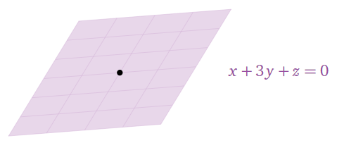
Figure \(\PageIndex{1}\)
(A subspace also turns out to be the same thing as the solution set of a homogeneous system of equations.)
Subspaces: Definition and Examples
A subset of \(\mathbb{R}^n\) is any collection of points of \(\mathbb{R}^n\).
Let \(U\) be a set of vectors in \(\mathbb{R}^n\). Then we say that \(U\) is a subset of \(\mathbb{R}^n\), denoted \[U \subset \mathbb{R}^n\nonumber \]
For instance, the unit circle
\[ C = \bigl\{ (x,y)\text{ in }\mathbb{R}^2 \bigm| x^2 + y^2 = 1 \bigr\} \nonumber \]
is a subset of \(\mathbb{R}^2\).
Above we expressed \(C\) in set builder notation, Note 2.2.3 in Section 2.2: in English, it reads “\(C\) is the set of all ordered pairs \((x,y)\) in \(\mathbb{R}^2\) such that \(x^2+y^2=1\).”
A subspace of \(\mathbb{R}^n\) is a subset \(V\) of \(\mathbb{R}^n\) satisfying:
- Non-emptiness: The zero vector is in \(V\).
- Closure under addition: If \(u\) and \(v\) are in \(V\text{,}\) then \(u+v\) is also in \(V\).
- Closure under scalar multiplication: If \(v\) is in \(V\) and \(c\) is in \(\mathbb{R}\text{,}\) then \(cv\) is also in \(V\).
As a consequence of these properties, we see:
- If \(v\) is a vector in \(V\text{,}\) then all scalar multiples of \(v\) are in \(V\) by the third property. In other words the line through any nonzero vector in \(V\) is also contained in \(V\).
- If \(u,v\) are vectors in \(V\) and \(c,d\) are scalars, then \(cu,dv\) are also in \(V\) by the third property, so \(cu+dv\) is in \(V\) by the second property. Therefore, all of \(\text{Span}\{u,v\}\) is contained in \(V\)
- Similarly, if \(v_1,v_2,\ldots,v_n\) are all in \(V\text{,}\) then \(\text{Span}\{v_1,v_2,\ldots,v_n\}\) is contained in \(V\). In other words, a subspace contains the span of any vectors in it.
If you choose enough vectors, then eventually their span will fill up \(V\text{,}\) so we already see that a subspace is a span. See this Theorem \(\PageIndex{1}\) below for a precise statement.
A quick test to determine whether a subset \(V \subseteq \mathbb{R}^n\) is a subspace is:
- The zero vector \(0\) is in \(V\).
- For any vectors \(v_1, v_2 \text{ in } V\) and any scalars \(c, d\), the linear combination
\[ c v_1 - d v_2 \text{ in } V. \]
The set \(\mathbb{R}^n\) is a subspace of itself: indeed, it contains zero, and is closed under addition and scalar multiplication.
The set \(\{0\}\) containing only the zero vector is a subspace of \(\mathbb{R}^n\text{:}\) it contains zero, and if you add zero to itself or multiply it by a scalar, you always get zero.
A line \(L\) through the origin is a subspace.
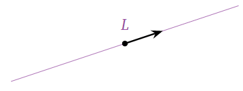
Figure \(\PageIndex{2}\)
Indeed, \(L\) contains zero, and is easily seen to be closed under addition and scalar multiplication.
A plane \(P\) through the origin is a subspace.
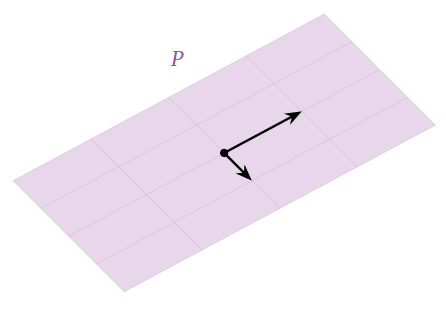
Figure \(\PageIndex{3}\)
Indeed, \(P\) contains zero; the sum of two vectors in \(P\) is also in \(P\text{;}\) and any scalar multiple of a vector in \(P\) is also in \(P\).
A line \(L\) (or any other subset) that does not contain the origin is not a subspace. It fails the first defining property: every subspace contains the origin by definition.
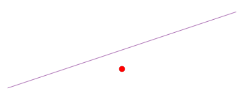
Figure \(\PageIndex{4}\)
The unit circle \(C\) is not a subspace. It fails all three defining properties: it does not contain the origin, it is not closed under addition, and it is not closed under scalar multiplication. In the picture, one red vector is the sum of the two black vectors (which are contained in \(C\)), and the other is a scalar multiple of a black vector.
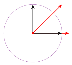
Figure \(\PageIndex{5}\)
The first quadrant in \(\mathbb{R}^2\) is not a subspace. It contains the origin and is closed under addition, but it is not closed under scalar multiplication (by negative numbers).
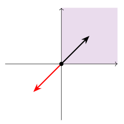
Figure \(\PageIndex{6}\)
The union of a line and a plane in \(\mathbb{R}^3\) is not a subspace. It contains the origin and is closed under scalar multiplication, but it is not closed under addition: the sum of a vector on the line and a vector on the plane is not contained in the line or in the plane.
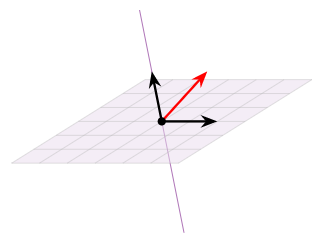
Figure \(\PageIndex{7}\)
A subset of \(\mathbb{R}^n\) is any collection of vectors whatsoever. For instance, the unit circle
\[ C = \bigl\{ (x,y)\text{ in }\mathbb{R}^2 \bigm| x^2 + y^2 = 1 \bigr\} \nonumber \]
is a subset of \(\mathbb{R}^2\text{,}\) but it is not a subspace. In fact, all of the non-examples above are still subsets of \(\mathbb{R}^n\). A subspace is a subset that happens to satisfy the three additional defining properties.
In order to verify that a subset of \(\mathbb{R}^n\) is in fact a subspace, one has to check the three defining properties. That is, unless the subset has already been verified to be a subspace: see this important note, Note \(\PageIndex{3}\), below.
Let
\[V=\left\{\left(\begin{array}{c}a\\b\end{array}\right)\text{ in }\mathbb{R}^{2}|2a=3b\right\}.\nonumber\]
Verify that \(V\) is a subspace.
Solution
First we point out that the condition “\(2a = 3b\)” defines whether or not a vector is in \(V\text{:}\) that is, to say \({a\choose b}\) is in \(V\) means that \(2a = 3b\). In other words, a vector is in \(V\) if twice its first coordinate equals three times its second coordinate. So for instance, \({3\choose 2}\) and \({1/2\choose 1/3}\) are in \(V\text{,}\) but \({2\choose 3}\) is not because \(2\cdot 2\neq 3\cdot 3\).
Let us check the first property. The subset \(V\) does contain the zero vector \({0\choose 0}\text{,}\) because \(2\cdot 0 = 3\cdot 0\).
Next we check the second property. To show that \(V\) is closed under addition, we have to check that for any vectors \(u = {a\choose b}\) and \(v = {c\choose d}\) in \(V\text{,}\) the sum \(u+v\) is in \(V\). Since we cannot assume anything else about \(u\) and \(v\text{,}\) we must treat them as unknowns.
We have
\[\left(\begin{array}{c}a\\b\end{array}\right)+\left(\begin{array}{c}c\\d\end{array}\right)=\left(\begin{array}{c}a+c\\b+d\end{array}\right).\nonumber\]
To say that \(a+c\choose b+d\) is contained in \(V\) means that \(2(a+c) = 3(b+d)\text{,}\) or \(2a + 2c = 3b + 3d\). The one thing we are allowed to assume about \(u\) and \(v\) is that \(2a = 3b\) and \(2c = 3d\text{,}\) so we see that \(u+v\) is indeed contained in \(V\).
Next we check the third property. To show that \(V\) is closed under scalar multiplication, we have to check that for any vector \(v = {a\choose b}\) in \(V\) and any scalar \(c\) in \(\mathbb{R}\text{,}\) the product \(cv\) is in \(V\). Again, we must treat \(v\) and \(c\) as unknowns. We have
\[c\left(\begin{array}{c}a\\b\end{array}\right)=\left(\begin{array}{c}ca\\cb\end{array}\right).\nonumber\]
To say that \(ca\choose cb\) is contained in \(V\) means that \(2(ca) = 3(cb)\text{,}\) i.e., that \(c\cdot 2a = c\cdot 3b\). The one thing we are allowed to assume about \(v\) is that \(2a = 3b\text{,}\) so \(cv\) is indeed contained in \(V\).
Since \(V\) satisfies all three defining properties, it is a subspace. In fact, it is the line through the origin with slope \(2/3\).
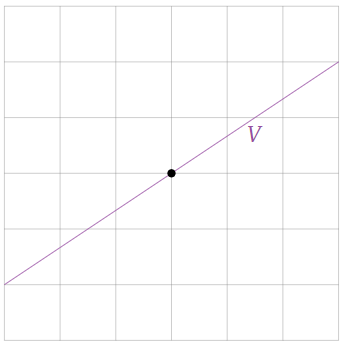
Figure \(\PageIndex{8}\)
Let
\[V=\left\{\left(\begin{array}{c}a\\b\end{array}\right)\text{ in }\mathbb{R}^{2}|ab=0\right\}.\nonumber\]
Is \(V\) a subspace?
Solution
First we point out that the condition “\(ab=0\)” defines whether or not a vector is in \(V\text{:}\) that is, to say \({a\choose b}\) is in \(V\) means that \(ab=0\). In other words, a vector is in \(V\) if the product of its coordinates is zero, i.e., if one (or both) of its coordinates are zero. So for instance, \({1\choose 0}\) and \({0\choose 2}\) are in \(V\text{,}\) but \({1\choose 1}\) is not because \(1\cdot 1\neq 0\).
Let us check the first property. The subset \(V\) does contain the zero vector \({0\choose 0}\text{,}\) because \(0\cdot 0=0\).
Next we check the third property. To show that \(V\) is closed under scalar multiplication, we have to check that for any vector \(v = {a\choose b}\) in \(V\) and any scalar \(c\) in \(\mathbb{R}\text{,}\) the product \(cv\) is in \(V\). Since we cannot assume anything else about \(v\) and \(c\text{,}\) we must treat them as unknowns.
We have
\[c\left(\begin{array}{c}a\\b\end{array}\right)=\left(\begin{array}{c}ca\\cb\end{array}\right).\nonumber\]
To say that \(ca\choose cb\) is contained in \(V\) means that \((ca)(cb)=0\). Rewriting, this means \(c^2(ab)=0\). The one thing we are allowed to assume about \(v\) is that \(ab=0\text{,}\) so we see that \(cv\) is indeed contained in \(V\).
Next we check the second property. It turns out that \(V\) is not closed under addition; to verify this, we must show that there exists some vectors \(u,v\) in \(V\) such that \(u+v\) is not contained in \(V\). The easiest way to do so is to produce examples of such vectors. We can take \(u={1\choose 0}\) and \(v={0\choose 1}\text{;}\) these are contained in \(V\) because the products of their coordinates are zero, but
\[\left(\begin{array}{c}1\\0\end{array}\right)+\left(\begin{array}{c}0\\1\end{array}\right)=\left(\begin{array}{c}1\\1\end{array}\right)\nonumber\]
is not contained in \(V\) because \(1\cdot 1\neq 0\).
Since \(V\) does not satisfy the second property (it is not closed under addition), we conclude that \(V\) is not a subspace. Indeed, it is the union of the two coordinate axes, which is not a span.
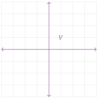
Figure \(\PageIndex{9}\)
Common Types of Subspaces
Let \(v_1, v_2, \ldots, v_k\) be vectors in a vector space \(V\), and let
\(c_1, c_2, \ldots, c_k\) be scalars.
A vector of the form
\[
c_1 v_1 + c_2 v_2 + \cdots + c_k v_k
\]
is called a linear combination of the vectors \(v_1, v_2, \ldots, v_k\).
If we are given a set of vectors, we can create infinitely many vectors from the linear combination formal.
Consider the vectors
\[
\mathbf{v}_1 = \begin{pmatrix} 1 \\ 2 \\ 0 \end{pmatrix},
\qquad
\mathbf{v}_2 = \begin{pmatrix} -1 \\ 0 \\ 3 \end{pmatrix},
\qquad
\mathbf{v}_3 = \begin{pmatrix} 2 \\ -1 \\ 1 \end{pmatrix}.
\]
A linear combination of these vectors is obtained by choosing scalars
\(c_1 = 2\), \(c_2 = -1\), and \(c_3 = 4\), giving
\[
2\mathbf{v}_1 - \mathbf{v}_2 + 4\mathbf{v}_3
= 2\begin{pmatrix} 1 \\ 2 \\ 0 \end{pmatrix}
- \begin{pmatrix} -1 \\ 0 \\ 3 \end{pmatrix}
+ 4\begin{pmatrix} 2 \\ -1 \\ 1 \end{pmatrix}
= \begin{pmatrix} 11 \\ 0 \\ 1 \end{pmatrix}.
\]
Thus,
\[
\mathbf{w}\begin{pmatrix} 11 \\ 0 \\ 1 \end{pmatrix}
\]
is a linear combination of \(\mathbf{v}_1, \mathbf{v}_2,\) and \(\mathbf{v}_3\).
The set that includes all of these vectors is defining bellow.
The collection of all linear combinations of a set of vectors \(\{ \vec{u}_1, \cdots ,\vec{u}_k\}\) in \(\mathbb{R}^{n}\) is known as the span of these vectors and is written as \(\mathrm{span} \{\vec{u}_1, \cdots , \vec{u}_k\}\).
Consider the following example.
Describe the span of the vectors \(\vec{u}=\left[ \begin{array}{rrr} 1 & 1 & 0 \end{array} \right]^T\) and \(\vec{v}=\left[ \begin{array}{rrr} 3 & 2 & 0 \end{array} \right]^T \in \mathbb{R}^{3}\).
Solution
You can see that any linear combination of the vectors \(\vec{u}\) and \(\vec{v}\) yields a vector of the form \(\left[ \begin{array}{rrr} x & y & 0 \end{array} \right]^T\) in the \(XY\)-plane.
Moreover every vector in the \(XY\)-plane is in fact such a linear combination of the vectors \(\vec{u}\) and \(\vec{v}\). That’s because \[\left[ \begin{array}{r} x \\ y \\ 0 \end{array} \right] = (-2x+3y) \left[ \begin{array}{r} 1 \\ 1 \\ 0 \end{array} \right] + (x-y)\left[ \begin{array}{r} 3 \\ 2 \\ 0 \end{array} \right]\nonumber \]
Thus \(\mathrm{span}\{\vec{u},\vec{v}\}\) is precisely the \(XY\)-plane. This concept is explained below in a interactive video format. Feel free to click on it and see the theory in action.
You can convince yourself that no single vector can span the \(XY\)-plane. In fact, take a moment to consider what is meant by the span of a single vector.
However you can make the set larger if you wish. For example consider the larger set of vectors \(\{ \vec{u}, \vec{v}, \vec{w}\}\) where \(\vec{w}=\left[ \begin{array}{rrr} 4 & 5 & 0 \end{array} \right]^T\). Since the first two vectors already span the entire \(XY\)-plane, the span is once again precisely the \(XY\)-plane and nothing has been gained. Of course if you add a new vector such as \(\vec{w}=\left[ \begin{array}{rrr} 0 & 0 & 1 \end{array} \right]^T\) then it does span a different space. What is the span of \(\vec{u}, \vec{v}, \vec{w}\) in this case?
The distinction between the sets \(\{ \vec{u}, \vec{v}\}\) and \(\{ \vec{u}, \vec{v}, \vec{w}\}\) will be made using the concept of linear independence.
Consider the vectors \(\vec{u}, \vec{v}\), and \(\vec{w}\) discussed above. In the next example, we will show how to formally demonstrate that \(\vec{w}\) is in the span of \(\vec{u}\) and \(\vec{v}\).
If \(v_1,v_2,\ldots,v_p\) are any vectors in \(\mathbb{R}^n\text{,}\) then \(\text{Span}\{v_1,v_2,\ldots,v_p\}\) is a subspace of \(\mathbb{R}^n\). Moreover, any subspace of \(\mathbb{R}^n\) can be written as a span of a set of \(p\) linearly independent vectors in \(\mathbb{R}^n\) for \(p\leq n\).
- Proof
-
To show that \(\text{Span}\{v_1,v_2,\ldots,v_p\}\) is a subspace, we have to verify the three defining properties.
- The zero vector \(0 = 0v_1 + 0v_2 + \cdots + 0v_p\) is in the span.
- If \(u = a_1v_1 + a_2v_2 + \cdots + a_pv_p\) and \(v = b_1v_1 + b_2v_2 + \cdots + b_pv_p\) are in \(\text{Span}\{v_1,v_2,\ldots,v_p\}\text{,}\) then
\[ u + v = (a_1+b_1)v_1 + (a_2+b_2)v_2 + \cdots + (a_p+b_p)v_p \nonumber \]
is also in \(\text{Span}\{v_1,v_2,\ldots,v_p\}\). - If \(v = a_1v_1 + a_2v_2 + \cdots + a_pv_p\) is in \(\text{Span}\{v_1,v_2,\ldots,v_p\}\) and \(c\) is a scalar, then
\[ cv = ca_1v_1 + ca_2v_2 + \cdots + ca_pv_p \nonumber \]
is also in \(\text{Span}\{v_1,v_2,\ldots,v_p\}\).
Since \(\text{Span}\{v_1,v_2,\ldots,v_p\}\) satisfies the three defining properties of a subspace, it is a subspace.
Now let \(V\) be a subspace of \(\mathbb{R}^n\). If \(V\) is the zero subspace, then it is the span of the empty set, so we may assume \(V\) is nonzero. Choose a nonzero vector \(v_1\) in \(V\). If \(V = \text{Span}\{v_1\}\text{,}\) then we are done. Otherwise, there exists a vector \(v_2\) that is in \(V\) but not in \(\text{Span}\{v_1\}\). Then \(\text{Span}\{v_1,v_2\}\) is contained in \(V\text{,}\) and by the increasing span criterion in Section 2.5, Theorem 2.5.2, the set \(\{v_1,v_2\}\) is linearly independent. If \(V = \text{Span}\{v_1,v_2\}\) then we are done. Otherwise, we continue in this fashion until we have written \(V = \text{Span}\{v_1,v_2,\ldots,v_p\}\) for some linearly independent set \(\{v_1,v_2,\ldots,v_p\}\). This process terminates after at most \(n\) steps by this important note in Section 2.5, Note 2.5.2.
If \(V = \text{Span}\{v_1,v_2,\ldots,v_p\}\text{,}\) we say that \(V\) is the subspace spanned by or generated by the vectors \(v_1,v_2,\ldots,v_p\). We call \(\{v_1,v_2,\ldots,v_p\}\) a spanning set for \(V\).
Any matrix naturally gives rise to two subspaces.
Let \(A\) be an \(m\times n\) matrix.
- The column space of \(A\) is the subspace of \(\mathbb{R}^m\) spanned by the columns of \(A\). It is written \(\text{Col}(A)\).
- The null space of \(A\) is the subspace of \(\mathbb{R}^n\) consisting of all solutions of the homogeneous equation \(Ax=0\text{:}\)
\[ \text{Nul}(A) = \bigl\{ x \text{ in } \mathbb{R}^n\bigm| Ax=0 \bigr\}. \nonumber \]
The column space is defined to be a span, so it is a subspace by the above Theorem, Theorem \(\PageIndex{1}\). We need to verify that the null space is really a subspace. In Section 2.4 we already saw that the set of solutions of \(Ax=0\) is always a span, so the fact that the null spaces is a subspace should not come as a surprise.
We have to verify the three defining properties. To say that a vector \(v\) is in \(\text{Nul}(A)\) means that \(Av = 0\).
- The zero vector is in \(\text{Nul}(A)\) because \(A0=0\).
- Suppose that \(u,v\) are in \(\text{Nul}(A)\). This means that \(Au=0\) and \(Av=0\). Hence
\[A(u+v)=Au+Av=0+0=0\nonumber\]
by the linearity of the matrix-vector product in Section 2.3, Proposition 2.3.1. Therefore, \(u+v\) is in \(\text{Nul}(A)\). - Suppose that \(v\) is in \(\text{Nul}(A)\) and \(c\) is a scalar. Then
\[A(cv)=cAv=c\cdot 0=0\nonumber\] by the linearity of the matrix-vector product, Proposition 2.3.1 in Section 2.3, so \(cv\) is also in \(\text{Nul}(A)\).
Since \(\text{Nul}(A)\) satisfies the three defining properties of a subspace, it is a subspace.
Describe the column space and the null space of
\[A=\left(\begin{array}{cc}1&1\\1&1\\1&1\end{array}\right).\nonumber\]
Solution
The column space is the span of the columns of \(A\text{:}\)
\[\text{Col}(A)=\text{Span}\left\{\left(\begin{array}{c}1\\1\\1\end{array}\right),\:\left(\begin{array}{c}1\\1\\1\end{array}\right)\right\}=\text{Span}\left\{\left(\begin{array}{c}1\\1\\1\end{array}\right)\right\}.\nonumber\]
This is a line in \(\mathbb{R}^3\).
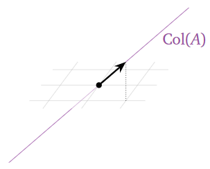
Figure \(\PageIndex{10}\)
The null space is the solution set of the homogeneous system \(Ax=0\). To compute this, we need to row reduce \(A\). Its reduced row echelon form is
\[\left(\begin{array}{cc}1&1\\0&0\\0&0\end{array}\right).\nonumber\]
This gives the equation \(x+y=0\text{,}\) or
\[\left\{\begin{array}{rrr}x &=& -y\\ y &=& y\end{array}\right. \quad\xrightarrow{\text{parametric vector form}}\quad \left(\begin{array}{c}x\\y\end{array}\right)=y\left(\begin{array}{c}-1\\1\end{array}\right).\nonumber\]
Hence the null space is \(\text{Span}\bigl\{{-1\choose 1}\bigr\}\text{,}\) which is a line in \(\mathbb{R}^2\).
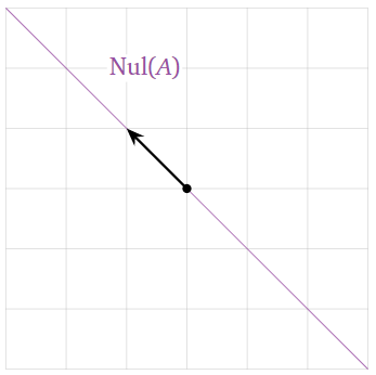
Figure \(\PageIndex{11}\)
Notice that the column space is a subspace of \(\mathbb{R}^3\text{,}\) whereas the null space is a subspace of \(\mathbb{R}^2\). This is because \(A\) has three rows and two columns.
The column space and the null space of a matrix are both subspaces, so they are both spans. The column space of a matrix \(A\) is defined to be the span of the columns of \(A\). The null space is defined to be the solution set of \(Ax=0\text{,}\) so this is a good example of a kind of subspace that we can define without any spanning set in mind. In other words, it is easier to show that the null space is a subspace than to show it is a span—see the proof above. In order to do computations, however, it is usually necessary to find a spanning set.
The null space of a matrix is the solution set of a homogeneous system of equations. For example, the null space of the matrix
\[A=\left(\begin{array}{ccc}1&7&2\\-2&1&3\\4&-2&-3\end{array}\right)\nonumber\]
is the solution set of \(Ax=0\text{,}\) i.e., the solution set of the system of equations
\[\left\{\begin{array}{rrrrrrl} x &+& 7y &+& 2z &=& 0\\ -2x &+& y &+& 3z &=& 0\\ 4x &-& 2y &-& 3z &=& 0.\end{array}\right.\nonumber\]
Conversely, the solution set of any homogeneous system of equations is precisely the null space of the corresponding coefficient matrix.
To find a spanning set for the null space, one has to solve a system of homogeneous equations.
To find a spanning set for \(\text{Nul}(A)\text{,}\) compute the parametric vector form of the solutions to the homogeneous equation \(Ax=0\). The vectors attached to the free variables form a spanning set for \(\text{Nul}(A)\).
Find a spanning set for the null space of the matrix
\[A=\left(\begin{array}{cccc}2&3&-8&-5 \\ -1&2&-3&-8\end{array}\right).\nonumber\]
Solution
We compute the parametric vector form of the solutions of \(Ax=0\). The reduced row echelon form of \(A\) is
\[\left(\begin{array}{cccc}1&0&-1&2 \\ 0&1&-2&-3\end{array}\right).\nonumber\]
The free variables are \(x_3\) and \(x_4\text{;}\) the parametric form of the solution set is
\[\left\{\begin{array}{rrrrr} x_1 &=& x_3 &-& 2x_4\\ x_2 &=& 2x_3 &+& 3x_4\\ x_3 &=& x_3&{}&{}\\ x_4 &=&{}&{}& x_4\end{array}\right. \quad\xrightarrow[\text{vector form}]{\text{parametric}}\quad \left(\begin{array}{c}x_1 \\x_2\\x_3\\x_4\end{array}\right)=x_3\left(\begin{array}{c}1\\2\\1\\0\end{array}\right)+x_4\left(\begin{array}{c}-2\\3\\0\\1\end{array}\right).\nonumber\]
Therefore,
\[\text{Nul}(A)=\text{Span}\left\{\left(\begin{array}{c}1\\2\\1\\0\end{array}\right),\:\left(\begin{array}{c}-2\\3\\0\\1\end{array}\right)\right\}.\nonumber\]
Find a spanning set for the null space of the matrix
\[A=\left(\begin{array}{cc}1&3\\2&4\end{array}\right).\nonumber\]
Solution
We compute the parametric vector form of the solutions of \(Ax=0\). The reduced row echelon form of \(A\) is
\[\left(\begin{array}{cc}1&0\\0&1\end{array}\right).\nonumber\]
There are no free variables; hence the only solution of \(Ax=0\) is the trivial solution. In other words,
\[\text{Nul}(A)=\{0\}=\text{Span}\{0\}.\nonumber\]
It is natural to define \(\text{Span}\{\} = \{0\}\text{,}\) so that we can take our spanning set to be empty. This is consistent with the definition of dimension, Definition 2.7.2, in Section 2.7.
Writing a subspace as a column space or a null space
A subspace can be given to you in many different forms. In practice, computations involving subspaces are much easier if your subspace is the column space or null space of a matrix. The simplest example of such a computation is finding a spanning set: a column space is by definition the span of the columns of a matrix, and we showed above how to compute a spanning set for a null space using parametric vector form. For this reason, it is useful to rewrite a subspace as a column space or a null space before trying to answer questions about it.
When asking questions about a subspace, it is usually best to rewrite the subspace as a column space or a null space.
This also applies to the question “is my subset a subspace?” If your subset is a column space or null space of a matrix, then the answer is yes.
Let
\[V=\left\{\left(\begin{array}{c}a\\b\end{array}\right)\text{ in }\mathbb{R}^{2}|2a=3b\right\}\nonumber\]
be the subset of a previous Example \(\PageIndex{9}\). The subset \(V\) is exactly the solution set of the homogeneous equation \(2x - 3y = 0\). Therefore,
\[V=\text{Nul} (2-3)\nonumber\]
In particular, it is a subspace. The reduced row echelon form of \(\left(\begin{array}{cc}2&-3\end{array}\right)\) is \(\left(\begin{array}{cc}1&-3/2\end{array}\right)\), so the parametric form of \(V\) is \(x = 3/2y\text{,}\) so the parametric vector form is \({x\choose y} = y{3/2\choose 1},\) and hence \(\bigl\{{3/2\choose 1}\bigr\}\) spans \(V\).
Let \(V\) be the plane in \(\mathbb{R}^3\) defined by
\[V=\left\{\left(\begin{array}{c}2x+y \\ x-y \\ 3x-2y \end{array}\right) |x,y\text{ are in }\mathbb{R}\right\}.\nonumber\]
Write \(V\) as the column space of a matrix.
Solution
Since
\[\left(\begin{array}{c}2x+y \\ x-y \\ 3x-2y\end{array}\right)=x\left(\begin{array}{c}2\\1\\3\end{array}\right)+y\left(\begin{array}{c}1\\-1\\-2\end{array}\right),\nonumber\]
we notice that \(V\) is exactly the span of the vectors
\[\left(\begin{array}{c}2\\1\\3\end{array}\right)\quad\text{and}\quad\left(\begin{array}{c}1\\-1\\-2\end{array}\right).\nonumber\]
Hence
\[V=\text{Col}\left(\begin{array}{cc}2&1\\1&-1\\3&-2\end{array}\right).\nonumber\]
Exercises
Let \(H=\mathrm{span}\left\{\left[\begin{array}{r}0\\2\\0\\-1\end{array}\right],\:\left[\begin{array}{r}-1\\6\\0\\-2\end{array}\right],\:\left[\begin{array}{r}-2\\16\\0\\-6\end{array}\right],\:\left[\begin{array}{r}-3\\22\\0\\-8\end{array}\right]\right\}\). Find the dimension of \(H\) and determine a basis.
Let \(H=\mathrm{span}\left\{\left[\begin{array}{r}5\\1\\1\\4\end{array}\right],\:\left[\begin{array}{r}14\\3\\2\\8\end{array}\right],\:\left[\begin{array}{r}38\\8\\6\\24\end{array}\right],\:\left[\begin{array}{r}47\\10\\7\\28\end{array}\right],\:\left[\begin{array}{r}10\\2\\3\\12\end{array}\right]\right\}\). Find the dimension of \(H\) and determine a basis.
Let \(H=\mathrm{span}\left\{\left[\begin{array}{r}6\\1\\1\\5\end{array}\right],\:\left[\begin{array}{r}17\\3\\2\\10\end{array}\right],\:\left[\begin{array}{r}52\\9\\7\\35\end{array}\right],\:\left[\begin{array}{r}18\\3\\4\\20\end{array}\right]\right\}\). Find the dimension of \(H\) and determine a basis.
Let \(M=\left\{\vec{u}=\left[\begin{array}{c}u_1 \\ u_2\\u_3\\u_4\end{array}\right]\in\mathbb{R}^4:\sin(u_1)=1\right\}\). Is \(M\) a subspace? Explain.
- Answer
-
No. Let \(\vec{u}=\left[\begin{array}{c}\frac{\pi}{2} \\ 0\\0\\0\end{array}\right]\). Then \(2\vec{u}\cancel{\in}M\) although \(\vec{u}\in M\).
Let \(M=\left\{\vec{u}=\left[\begin{array}{c}u_1 \\ u_2\\u_3\\u_4\end{array}\right]\in\mathbb{R}^4:||u_1||\leq 4\right\}\). Is \(M\) a subspace? Explain.
- Answer
-
No. \(\left[\begin{array}{c}1\\0\\0\\0\end{array}\right]\in M\) but \(10\left[\begin{array}{c}1\\0\\0\\0\end{array}\right]\cancel{\in }M\).
Let \(M=\left\{\vec{u}=\left[\begin{array}{c}u_1 \\ u_2\\u_3\\u_4\end{array}\right]\in\mathbb{R}^4:u_1\geq 0\text{ for each }i=1,2,3,4 \right\}\). Is \(M\) a subspace? Explain.
- Answer
-
This is not a subspace. \(\left[\begin{array}{c}1\\1\\1\\1\end{array}\right]\) is in it. However, \((-1)\left[\begin{array}{c}1\\1\\1\\1\end{array}\right]\) is not.
Let \(\vec{w}\), \(\vec{w}_1\) be given vectors in \(\mathbb{R}^4\) and define \[M=\left\{\vec{u}=\left[\begin{array}{c}u_1\\u_2\\u_3\\u_4\end{array}\right]\in\mathbb{R}^4 :\vec{w}\bullet\vec{u}=0\text{ and }\vec{w}_1\bullet\vec{u}=0\right\}.\nonumber\] Is \(M\) a subspace? Explain.
- Answer
-
This is a subspace because it is closed with respect to vector addition and scalar multiplication.
Let \(\vec{w}\in\mathbb{R}^4\) and let \(M=\left\{\vec{u}=\left[\begin{array}{c}u_1 \\ u_2\\u_3\\u_4\end{array}\right]\in\mathbb{R}^4:\vec{w}\bullet\vec{u}=0\right\}\). Is \(M\) a subspace? Explain.
- Answer
-
Yes, this is a subspace because it is closed with respect to vector addition and scalar multiplication.
Let \(M=\left\{\vec{u}=\left[\begin{array}{c}u_1 \\ u_2\\u_3\\u_4\end{array}\right]\in\mathbb{R}^4:u_3\geq u_1\right\}\). Is \(M\) a subspace? Explain.
- Answer
-
This is not a subspace. \(\left[\begin{array}{c}0\\0\\1\\0\end{array}\right]\) is in it. However \((-1)\left[\begin{array}{c}0\\0\\1\\0\end{array}\right]=\left[\begin{array}{r}0\\0\\-1\\0\end{array}\right]\) is not.
Let \(M=\left\{\vec{u}=\left[\begin{array}{c}u_1 \\ u_2\\u_3\\u_4\end{array}\right]\in\mathbb{R}^4:u_3=u_1=0\right\}\). Is \(M\) a subspace? Explain.
- Answer
-
This is a subspace. It is closed with respect to vector addition and scalar multiplication.
Consider the set of vectors \(S\) given by \[S=\left\{\left[\begin{array}{c}4u+v-5w \\ 12u+6v-6w \\ 4u+4v+4w\end{array}\right] :u,v,w\in\mathbb{R}\right\}.\nonumber\] Is \(S\) a subspace of \(\mathbb{R}^3\)?
Consider the set of vectors \(S\) given by \[S=\left\{\left[\begin{array}{c}2u+6v+7w \\ -3u-9v-12w \\ 2u+6v+6w \\ u+3v+3w \end{array}\right] :u,v,w\in\mathbb{R}\right\}.\nonumber\] Is \(S\) a subspace of \(\mathbb{R}^4\)?
Consider the set of vectors \(S\) given by \[S=\left\{\left[\begin{array}{c}2u+v \\ 6v-3u+3w \\ 3v-6u+3w \end{array}\right] :u,v,w\in\mathbb{R}\right\}.\nonumber\] Is this set of vectors a subspace of \(\mathbb{R}^3\)?
Consider the vectors of the form \[\left\{\left[\begin{array}{c}2u+v+7w \\ u-2v+w \\ -6v-6w \end{array}\right] :u,v,w\in\mathbb{R}\right\}.\nonumber\] Is this set of vectors a subspace of \(\mathbb{R}^3\)?
Consider the vectors of the form \[\left\{\left[\begin{array}{c}3u+v+11w \\ 18u+6v+66w \\ 28u+8v+100w \end{array}\right] :u,v,w\in\mathbb{R}\right\}.\nonumber\] Is this set of vectors a subspace of \(\mathbb{R}^3\)?
Consider the vectors of the form \[\left\{\left[\begin{array}{c}3u+v \\ 2w-4u \\ 2w-2v-8u \end{array}\right] :u,v,w\in\mathbb{R}\right\}.\nonumber\] Is this set of vectors a subspace of \(\mathbb{R}^3\)?
Consider the set of vectors \(S\) given by \[\left\{\left[\begin{array}{c}u+v+w \\ 2u+2v+4w \\ u+v+w \\ 0 \end{array}\right] :u,v,w\in\mathbb{R}\right\}.\nonumber\] Is \(S\) is a subspace of \(\mathbb{R}^4\)?
Consider the set of vectors \(S\) given by \[\left\{\left[\begin{array}{c}v \\ -3u-3w \\ 8u-4v+4w \end{array}\right] :u,v,w\in\mathbb{R}\right\}.\nonumber\] Is \(S\) is a subspace of \(\mathbb{R}^4\)?
If you have \(5\) vectors in \(\mathbb{R}^5\) and the vectors are linearly independent, can it always be concluded they span \(\mathbb{R}^5\)? Explain.
- Answer
-
Yes. If not, there would exist a vector not in the span. But then you could add in this vector and obtain a linearly independent set of vectors with more vectors than a basis.
If you have \(6\) vectors in \(\mathbb{R}^5\), is it possible they are linearly independent? Explain.
- Answer
-
They can't be.
Suppose \(A\) is an \(m\times n\) matrix and \(\{\vec{w}_1,\cdots ,\vec{w}_k\}\) is a linearly independent set of vectors in \(A(\mathbb{R}^n ) ⊆ \mathbb{R}^m\). Now suppose \(A\vec{z}_i = \vec{w}_i\). Show \(\{\vec{z}_1 ,\cdots ,\vec{z}_k\}\) is also independent.
- Answer
-
Say \(\sum\limits_{i=1}^k c_i\vec{z}_i=\vec{0}\). Then apply \(A\) to it as follows. \[\sum\limits_{i=1}^k c_aA\vec{z}_i=\sum\limits_{i=1}^kc_i\vec{w}_i=\vec{0}\nonumber\] and so, by linear independence of the \(\vec{w}_i\), it follows that each \(c_i=0\).
Let \(V\) and \(W\) be subspaces of \(\mathbb{R}^n\). Show that the intersection \(V \cap W\) is also a subspace of \(\mathbb{R}^n\)