16.2: Basic Classes of Functions

Last updated
Save as PDF

Page ID: 46402

$ \newcommand{\vecs}[1]{\overset { \scriptstyle \rightharpoonup} {\mathbf{#1}} } $ $ \newcommand{\vecd}[1]{\overset{-\!-\!\rightharpoonup}{\vphantom{a}\smash {#1}}} $$\newcommand{\id}{\mathrm{id}}$ $ \newcommand{\Span}{\mathrm{span}}$ $ \newcommand{\kernel}{\mathrm{null}\,}$ $ \newcommand{\range}{\mathrm{range}\,}$ $ \newcommand{\RealPart}{\mathrm{Re}}$ $ \newcommand{\ImaginaryPart}{\mathrm{Im}}$ $ \newcommand{\Argument}{\mathrm{Arg}}$ $ \newcommand{\norm}[1]{\| #1 \|}$ $ \newcommand{\inner}[2]{\langle #1, #2 \rangle}$ $ \newcommand{\Span}{\mathrm{span}}$ $\newcommand{\id}{\mathrm{id}}$ $ \newcommand{\Span}{\mathrm{span}}$ $ \newcommand{\kernel}{\mathrm{null}\,}$ $ \newcommand{\range}{\mathrm{range}\,}$ $ \newcommand{\RealPart}{\mathrm{Re}}$ $ \newcommand{\ImaginaryPart}{\mathrm{Im}}$ $ \newcommand{\Argument}{\mathrm{Arg}}$ $ \newcommand{\norm}[1]{\| #1 \|}$ $ \newcommand{\inner}[2]{\langle #1, #2 \rangle}$ $ \newcommand{\Span}{\mathrm{span}}$$\newcommand{\AA}{\unicode[.8,0]{x212B}}$

We have studied the general characteristics of functions, so now let’s examine some specific classes of functions. We begin by reviewing the basic properties of linear and quadratic functions, and then generalize to include higher-degree polynomials. By combining root functions with polynomials, we can define general algebraic functions and distinguish them from the transcendental functions we examine later in this chapter. We finish the section with examples of piecewise-defined functions and take a look at how to sketch the graph of a function that has been shifted, stretched, or reflected from its initial form.

Linear Functions and Slope

The easiest type of function to consider is a linear function. Linear functions have the form $f(x)=ax+b$, where $a$ and $b$ are constants. In Figure $\PageIndex{1}$, we see examples of linear functions when a is positive, negative, and zero. Note that if $a>0$, the graph of the line rises as $x$ increases. In other words, $f(x)=ax+b$ is increasing on $(−∞, ∞)$. If $a<0$, the graph of the line falls as $x$ increases. In this case, $f(x)=ax+b$ is decreasing on $(−∞, ∞)$. If $a=0$, the line is horizontal.

$CNX_Calc_Figure_01_02_001.jpeg$

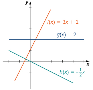
Figure $\PageIndex{1}$: These linear functions are increasing or decreasing on $(∞, ∞)$ and one function is a horizontal line.

As suggested by Figure, the graph of any linear function is a line. One of the distinguishing features of a line is its slope. The slope is the change in $y$ for each unit change in $x$. The slope measures both the steepness and the direction of a line. If the slope is positive, the line points upward when moving from left to right. If the slope is negative, the line points downward when moving from left to right. If the slope is zero, the line is horizontal. To calculate the slope of a line, we need to determine the ratio of the change in $y$ versus the change in $x$. To do so, we choose any two points $(x_1,y_1)$ and $(x_2,y_2)$ on the line and calculate $\dfrac{y_2−y_1}{x_2−x_1}$. In Figure $\PageIndex{2}$, we see this ratio is independent of the points chosen.

$CNX_Calc_Figure_01_02_021.jpeg$

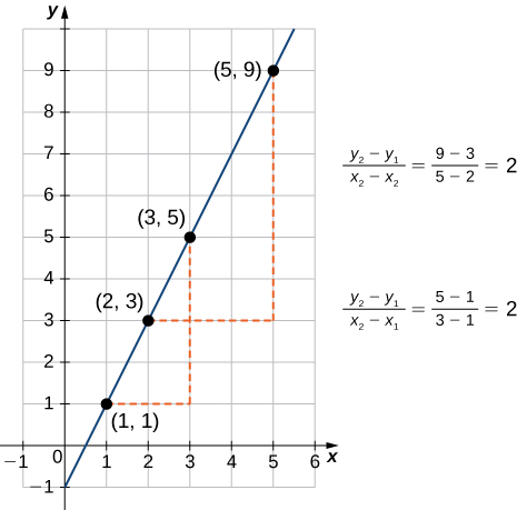
Figure $\PageIndex{2}$: For any linear function, the slope $(y_2−y_1)/(x_2−x_1)$ is independent of the choice of points $(x_1,y_1)$ and $(x_2,y_2)$ on the line.

Definition: Linear Functions

Consider line $L$ passing through points $(x_1,y_1)$ and $(x_2,y_2)$. Let $Δy=y_2−y_1$ and $Δx=x_2−x_1$ denote the changes in $y$ and $x$,respectively. The slope of the line is

\[m=\dfrac{y_2−y_1}{x_2−x_1}=\dfrac{Δy}{Δx}\]

We now examine the relationship between slope and the formula for a linear function. Consider the linear function given by the formula $f(x)=ax+b$. As discussed earlier, we know the graph of a linear function is given by a line. We can use our definition of slope to calculate the slope of this line. As shown, we can determine the slope by calculating $(y_2−y_1)/(x_2−x_1)$ for any points $(x_1,y_1)$ and $(x_2,y_2)$ on the line. Evaluating the function $f$ at $x=0$, we see that $(0,b)$ is a point on this line. Evaluating this function at $x=1$, we see that $(1,a+b)$ is also a point on this line. Therefore, the slope of this line is

\[\dfrac{(a+b)−b}{1−0}=a.\]

We have shown that the coefficient $a$ is the slope of the line. We can conclude that the formula $f(x)=ax+b$ describes a line with slope $a$. Furthermore, because this line intersects the $y$-axis at the point $(0,b)$, we see that the y-intercept for this linear function is $(0,b)$. We conclude that the formula $f(x)=ax+b$ tells us the slope, a, and the $y$-intercept, $(0,b)$, for this line. Since we often use the symbol $m$ to denote the slope of a line, we can write

\[f(x)=mx+b\]

to denote the slope-intercept form of a linear function.

Sometimes it is convenient to express a linear function in different ways. For example, suppose the graph of a linear function passes through the point $(x_1,y_1)$ and the slope of the line is $m$. Since any other point $(x,f(x))$ on the graph of $f$ must satisfy the equation

\[m=\dfrac{f(x)−y_1}{x−x_1},\]

this linear function can be expressed by writing

\[f(x)−y_1=m(x−x_1).\]

We call this equation the point-slope equation for that linear function.

Since every nonvertical line is the graph of a linear function, the points on a nonvertical line can be described using the slope-intercept or point-slope equations. However, a vertical line does not represent the graph of a function and cannot be expressed in either of these forms. Instead, a vertical line is described by the equation $x=k$ for some constant $k$. Since neither the slope-intercept form nor the point-slope form allows for vertical lines, we use the notation

\[ax+by=c,\]

where $a,b$ are both not zero, to denote the standard form of a line.

Definition: point-slope equation, point-slope equation and the standard form of a line

Consider a line passing through the point $(x_1,y_1)$ with slope $m$. The equation

\[y−y_1=m(x−x_1)\]

is the point-slope equation for that line.

Consider a line with slope $m$ and $y$-intercept $(0,b).$ The equation

\[y=mx+b\]

is an equation for that line in point-slope equation.

The standard form of a line is given by the equation

\[ax+by=c,\]

where $a$ and $b$ are both not zero. This form is more general because it allows for a vertical line, $x=k$.

Example $\PageIndex{1}$: Finding the Slope and Equations of Lines

Consider the line passing through the points $(11,−4)$ and $(−4,5)$, as shown in Figure.

$imageedit_2_6502522226.png$

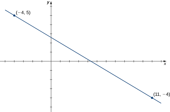
Figure $\PageIndex{3}$: Finding the equation of a linear function with a graph that is a line between two given points.

Find the slope of the line.
Find an equation for this linear function in point-slope form.
Find an equation for this linear function in slope-intercept form.

Solution

1. The slope of the line is

\[m=\dfrac{y_2−y_1}{x_2−x_1}=\dfrac{5−(−4)}{−4−11}=−\dfrac{9}{15}=−\dfrac{3}{5}.\]

2. To find an equation for the linear function in point-slope form, use the slope $m=−3/5$ and choose any point on the line. If we choose the point $(11,−4)$, we get the equation

\[f(x)+4=−\dfrac{3}{5}(x−11).\]

3. To find an equation for the linear function in slope-intercept form, solve the equation in part b. for $f(x)$. When we do this, we get the equation

\[f(x)=−\dfrac{3}{5}x+\dfrac{13}{5}.\]

Exercise $\PageIndex{1}$

Consider the line passing through points $(−3,2)$ and $(1,4)$.

Find the slope of the line.
Find an equation of that line in point-slope form.
Find an equation of that line in slope-intercept form.

Hint: The slope $m=Δy/Δx$.

Answer a: $m=1/2$.
Answer b: The point-slope form is $y−4=\dfrac{1}{2}(x−1)$.
Answer c: The slope-intercept form is $y=\dfrac{1}{2}x+\dfrac{7}{2}$.

Example $\PageIndex{2}$:

Jessica leaves her house at 5:50 a.m. and goes for a 9-mile run. She returns to her house at 7:08 a.m. Answer the following questions, assuming Jessica runs at a constant pace.

Describe the distance $D$ (in miles) Jessica runs as a linear function of her run time $t$ (in minutes).
Sketch a graph of $D$.
Interpret the meaning of the slope.

Solution:

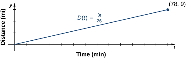
a. At time $t=0$, Jessica is at her house, so $D(0)=0$. At time $t=78$ minutes, Jessica has finished running $9$ mi, so $D(78)=9$. The slope of the linear function is

$m=\dfrac{9−0}{78−0}=\dfrac{3}{26}.$

The $y$-intercept is $(0,0)$, so the equation for this linear function is

$D(t)=\dfrac{3}{26}t.$

b. To graph $D$, use the fact that the graph passes through the origin and has slope $m=3/26.$

$imageedit_6_6266248475.png$

c. The slope $m=3/26≈0.115$ describes the distance (in miles) Jessica runs per minute, or her average velocity.

Polynomials

A linear function is a special type of a more general class of functions: polynomials. A polynomial function is any function that can be written in the form

\[f(x)=a_nx^n+a_{n−1}x^{n−1}+…+a_1x+a_0\]

for some integer $n≥0$ and constants $a_n,a+{n−1},…,a_0$, where $a_n≠0$. In the case when $n=0$, we allow for $a_0=0$; if $a_0=0$, the function $f(x)=0$ is called the zero function. The value $n$ is called the degree of the polynomial; the constant an is called the leading coefficient. A linear function of the form $f(x)=mx+b$ is a polynomial of degree 1 if $m≠0$ and degree 0 if $m=0$. A polynomial of degree 0 is also called a constant function. A polynomial function of degree 2 is called a quadratic function. In particular, a quadratic function has the form $f(x)=ax^2+bx+c$, where $a≠0$. A polynomial function of degree $3$ is called a cubic function.

Power Functions

Some polynomial functions are power functions. A power function is any function of the form $f(x)=ax^b$, where $a$ and $b$ are any real numbers. The exponent in a power function can be any real number, but here we consider the case when the exponent is a positive integer. (We consider other cases later.) If the exponent is a positive integer, then $f(x)=ax^n$ is a polynomial. If $n$ is even, then $f(x)=ax^n$ is an even function because $f(−x)=a(−x)^n=ax^n$ if $n$ is even. If $n$ is odd, then $f(x)=ax^n$ is an odd function because $f(−x)=a(−x)^n=−ax^n$ if $n$ is odd (Figure $\PageIndex{3}$).

$CNX_Calc_Figure_01_02_004.jpeg$

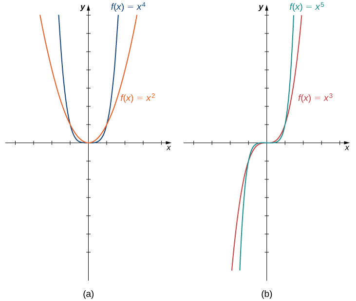
Figure $\PageIndex{4}$: (a) For any even integer $n$,$f(x)=ax^n$ is an even function. (b) For any odd integer $n$,$f(x)=ax^n$ is an odd function.

Mathematical Models

A large variety of real-world situations can be described using mathematical models. A mathematical model is a method of simulating real-life situations with mathematical equations. Physicists, engineers, economists, and other researchers develop models by combining observation with quantitative data to develop equations, functions, graphs, and other mathematical tools to describe the behavior of various systems accurately. Models are useful because they help predict future outcomes. Examples of mathematical models include the study of population dynamics, investigations of weather patterns, and predictions of product sales.

As an example, let’s consider a mathematical model that a company could use to describe its revenue for the sale of a particular item. The amount of revenue $R$ a company receives for the sale of n items sold at a price of $p$ dollars per item is described by the equation $R=p⋅n$. The company is interested in how the sales change as the price of the item changes. Suppose the data in Table show the number of units a company sells as a function of the price per item.

*Number of Units Sold $n$ (in Thousands) as a Function of Price per Unit $p$ (in Dollars)*
$p$	6	8	10	12	14
$n$	19.4	18.5	16.2	13.8	12.2

In Figure, we see the graph the number of units sold (in thousands) as a function of price (in dollars). We note from the shape of the graph that the number of units sold is likely a linear function of price per item, and the data can be closely approximated by the linear function $n= −1.04p+26$ for $0≤p≤25$, where $n$ predicts the number of units sold in thousands. Using this linear function, the revenue (in thousands of dollars) can be estimated by the quadratic function

\[R(p)=p⋅ (−1.04p+26)=−1.04p^2+26p\]

for $0≤p≤25$ In Example $\PageIndex{1}$, we use this quadratic function to predict the amount of revenue the company receives depending on the price the company charges per item. Note that we cannot conclude definitively the actual number of units sold for values of $p$, for which no data are collected. However, given the other data values and the graph shown, it seems reasonable that the number of units sold (in thousands) if the price charged is $p$ dollars may be close to the values predicted by the linear function $n=−1.04p+26.$

$CNX_Calc_Figure_01_02_008.jpeg$

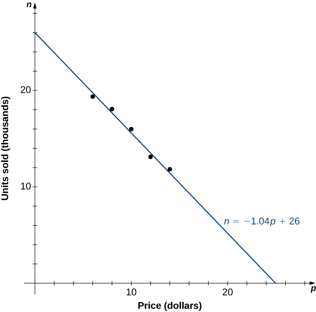
Figure $\PageIndex{6}$: The data collected for the number of items sold as a function of price is roughly linear. We use the linear function $n=−1.04p+26$ to estimate this function.

Algebraic Functions

By allowing for quotients and fractional powers in polynomial functions, we create a larger class of functions. An algebraic function is one that involves addition, subtraction, multiplication, division, rational powers, and roots. Two types of algebraic functions are rational functions and root functions.

Just as rational numbers are quotients of integers, rational functions are quotients of polynomials. In particular, a rational function is any function of the form $f(x)=p(x)/q(x)$,where $p(x)$ and $q(x)$ are polynomials. For example,

$f(x)=\dfrac{3x−1}{5x+2}$ and $g(x)=\dfrac{4}{x^2+1}$

are rational functions. A root function is a power function of the form $f(x)=x^{1/n}$, where n is a positive integer greater than one. For example, f(x)=x1/2=x√ is the square-root function and $g(x)=x^{1/3}=\sqrt[3]{x})$ is the cube-root function. By allowing for compositions of root functions and rational functions, we can create other algebraic functions. For example, $f(x)=\sqrt{4−x^2}$ is an algebraic function.

Example $\PageIndex{5}$: Finding Domain and Range for Algebraic Functions

For each of the following functions, find the domain and range.

$f(x)=\dfrac{3x−1}{5x+2}$
$f(x)=\sqrt{4−x^2}$

Solution

1.It is not possible to divide by zero, so the domain is the set of real numbers $x$ such that $x≠−2/5$. To find the range, we need to find the values $y$ for which there exists a real number $x$ such that

$y=\dfrac{3x−1}{5x+2}$

When we multiply both sides of this equation by $5x+2$, we see that $x$ must satisfy the equation

$5xy+2y=3x−1.$

From this equation, we can see that $x$ must satisfy

$2y+1=x(3−5y).$

If y=$3/5$, this equation has no solution. On the other hand, as long as $y≠3/5$,

$x=\dfrac{2y+1}{3−5y}$

satisfies this equation. We can conclude that the range of $f$ is ${y|y≠3/5}$.

2. To find the domain of $f$, we need $4−x^2≥0$. When we factor, we write $4−x^2=(2−x)(2+x)≥0$. This inequality holds if and only if both terms are positive or both terms are negative. For both terms to be positive, we need to find $x$ such that

$2−x≥0$ and $2+x≥0.$

These two inequalities reduce to $2≥x$ and $x≥−2$. Therefore, the set ${x|−2≤x≤2}$ must be part of the domain. For both terms to be negative, we need

$2−x≤0$ and $2+x≥0.$

These two inequalities also reduce to $2≤x$ and $x≥−2$. There are no values of $x$ that satisfy both of these inequalities. Thus, we can conclude the domain of this function is ${x|−2≤x≤2}.$

If $−2≤x≤2$, then $0≤4−x^2≤4$. Therefore, $0≤\sqrt{4−x2}≤2$, and the range of $f$ is ${y|0≤y≤2}.$

Exercise $\PageIndex{3}$

Find the domain and range for the function $f(x)=(5x+2)/(2x−1).$

Hint: The denominator cannot be zero. Solve the equation $y=(5x+2)/(2x−1)$ for $x$ to find the range.
Answer: The domain is the set of real numbers $x$ such that $x≠1/2$. The range is the set $\{y|y≠5/2\}$.

The root functions $f(x)=x^{1/n}$ have defining characteristics depending on whether $n$ is odd or even. For all even integers $n≥2$, the domain of $f(x)=x^{1/n}$ is the interval $[0,∞)$. For all odd integers $n≥1$, the domain of $f(x)=x^{1/n}$ is the set of all real numbers. Since $x^{1/n}=(−x)^{1/n}$ for odd integers $n$ ,$f(x)=x^{1/n}$ is an odd function if$n$ is odd. See the graphs of root functions for different values of $n$ in Figure.

$CNX_Calc_Figure_01_02_022.jpeg$

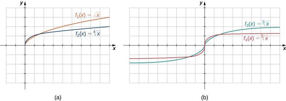
Figure $\PageIndex{7}$: (a) If $n$ is even, the domain of $f(x)=\sqrt[n]{x}$ is $[0,∞)$. (b) If $n$ is odd, the domain of $f(x)=\dfrac[n]{x}$ is $(−∞,∞)$ and the function $f(x)=\dfrac[n]{x}$ is an odd function.

Example $\PageIndex{6}$: Finding Domains for Algebraic Functions

For each of the following functions, determine the domain of the function.

$f(x)=\dfrac{3}{x^2−1}$
$f(x)=\dfrac{2x+5}{3x^2+4}$
$f(x)=\sqrt{4−3x}$
$f(x)=\sqrt[3]{2x−1}$

Solution

You cannot divide by zero, so the domain is the set of values $x$ such that $x^2−1≠0$. Therefore, the domain is ${x|x≠±1}$.
You need to determine the values of $x$ for which the denominator is zero. Since $3x^2+4≥4$ for all real numbers $x$, the denominator is never zero. Therefore, the domain is $(−∞,∞).$
Since the square root of a negative number is not a real number, the domain is the set of values $x$ for which $4−3x≥0$. Therefore, the domain is ${x|x≤4/3}.$
The cube root is defined for all real numbers, so the domain is the interval $(−∞, ∞).$

Exercise $\PageIndex{4}$

Find the domain for each of the following functions: $f(x)=(5−2x)/(x^2+2)$ and $g(x)=\sqrt{5x−1}$.

Hint: Determine the values of $x$ when the expression in the denominator of $f$ is nonzero, and find the values of $x$ when the expression inside the radical of $g$ is nonnegative.

Answer: The domain of $f$ is $(−∞, ∞)$. The domain of $g$ is ${x|x≥1/5}.$

Transformations of Functions

We have seen several cases in which we have added, subtracted, or multiplied constants to form variations of simple functions. In the previous example, for instance, we subtracted 2 from the argument of the function $y=x^2$ to get the function$ f(x)=(x−2)^2). This subtraction represents a shift of the function \(y=x^2$ two units to the right. A shift, horizontally or vertically, is a type of transformation of a function. Other transformations include horizontal and vertical scalings, and reflections about the axes.

A vertical shift of a function occurs if we add or subtract the same constant to each output $y$. For $c>0$, the graph of $f(x)+c$ is a shift of the graph of $f(x)$ up c units, whereas the graph of $f(x)−c$ is a shift of the graph of $f(x)$ down $c$ units. For example, the graph of the function $f(x)=x^3+4$ is the graph of $y=x^3$ shifted up $4$ units; the graph of the function $f(x)=x^3−4$ is the graph of $y=x^3$ shifted down $4$ units (Figure $\PageIndex{6}$).

$CNX_Calc_Figure_01_02_023.jpeg$

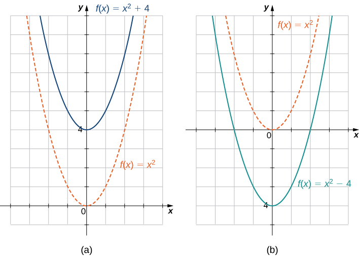
Figure $\PageIndex{9}$: (a) For $c>0$, the graph of $y=f(x)+c$ is a vertical shift up $c$ units of the graph of $y=f(x)$. (b) For $c>0$, the graph of $y=f(x)−c$ is a vertical shift down c units of the graph of $y=f(x)$.

A horizontal shift of a function occurs if we add or subtract the same constant to each input $x$. For $c>0$, the graph of $f(x+c)$ is a shift of the graph of $f(x)$ to the left $c$ units; the graph of $f(x−c)$ is a shift of the graph of $f(x)$ to the right $c$ units. Why does the graph shift left when adding a constant and shift right when subtracting a constant? To answer this question, let’s look at an example.

Consider the function $f(x)=|x+3|$ and evaluate this function at $x−3$. Since $f(x−3)=|x|$ and $x−3<x$, the graph of $f(x)=|x+3|$ is the graph of $y=|x|$ shifted left $3$ units. Similarly, the graph of $f(x)=|x−3|$ is the graph of $y=|x|$ shifted right $3$ units (Figure $\PageIndex{7}$).

$CNX_Calc_Figure_01_02_015.jpeg$

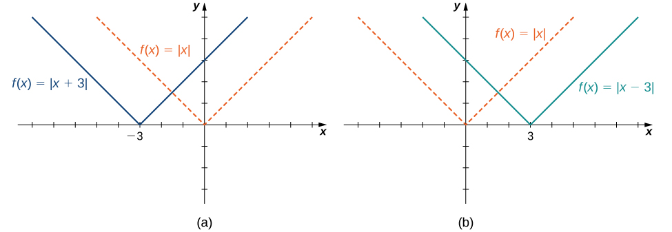
Figure $\PageIndex{10}$: (a) For $c>0$, the graph of $y=f(x+c)$ is a horizontal shift left $c$ units of the graph of $y=f(x)$. (b) For $c>0$, the graph of $y=f(x−c)$ is a horizontal shift right $c$ units of the graph of $y=f(x).$

A vertical scaling of a graph occurs if we multiply all outputs $y$ of a function by the same positive constant. For $c>0$, the graph of the function $cf(x)$ is the graph of $f(x)$ scaled vertically by a factor of $c$. If $c>1$, the values of the outputs for the function $cf(x)$ are larger than the values of the outputs for the function $f(x)$; therefore, the graph has been stretched vertically. If $0<c<1$, then the outputs of the function $cf(x)$ are smaller, so the graph has been compressed. For example, the graph of the function $f(x)=3x^2$ is the graph of $y=x^2$ stretched vertically by a factor of 3, whereas the graph of $f(x)=x^2/3$ is the graph of $y=x^2$ compressed vertically by a factor of $3$ (Figure $\PageIndex{8}$).

$CNX_Calc_Figure_01_02_024.jpeg$

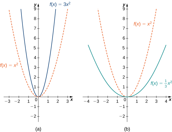
Figure $\PageIndex{11}$: (a) If $c>1$, the graph of $y=cf(x)$ is a vertical stretch of the graph of $y=f(x)$. (b) If $0<c<1$, the graph of $y=cf(x)$ is a vertical compression of the graph of $y=f(x)$.

The horizontal scaling of a function occurs if we multiply the inputs $x$ by the same positive constant. For $c>0$, the graph of the function $f(cx)$ is the graph of $f(x)$ scaled horizontally by a factor of $c$. If $c>1$, the graph of $f(cx)$ is the graph of $f(x)$ compressed horizontally. If $0<c<1$, the graph of $f(cx)$ is the graph of $f(x)$ stretched horizontally. For example, consider the function $f(x)=\sqrt{2x}$ and evaluate $f$ at $x/2$. Since $f(x/2)=\sqrt{x}$, the graph of $f(x)=\sqrt{2x}$ is the graph of $y=\sqrt{x}$ compressed horizontally. The graph of $y=\sqrt{x/2}$ is a horizontal stretch of the graph of $y=\sqrt{x}$ (Figure $\PageIndex{9}$).

$CNX_Calc_Figure_01_02_017.jpeg$

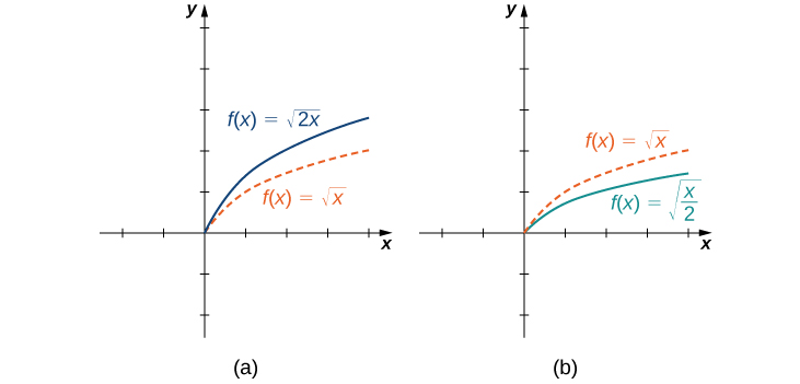
Figure $\PageIndex{12}$: (a) If $c>1$, the graph of $y=f(cx)$ is a horizontal compression of the graph of $y=f(x)$. (b) If $0<c<1$, the graph of $y=f(cx)$ is a horizontal stretch of the graph of $y=f(x)$.

We have explored what happens to the graph of a function $f$ when we multiply $f$ by a constant $c>0$ to get a new function $cf(x)$. We have also discussed what happens to the graph of a function $f$when we multiply the independent variable $x$ by $c>0$ to get a new function $f(cx)$. However, we have not addressed what happens to the graph of the function if the constant $c$ is negative. If we have a constant $c<0), we can write \(c$ as a positive number multiplied by $−1$; but, what kind of transformation do we get when we multiply the function or its argument by $−1?$ When we multiply all the outputs by $−1$, we get a reflection about the $x$-axis. When we multiply all inputs by $−1$, we get a reflection about the $y$-axis. For example, the graph of $f(x)=−(x^3+1)$ is the graph of $y=(x^3+1)$ reflected about the $x$-axis. The graph of $f(x)=(−x)^3+1$ is the graph of $y=x^3+1$ reflected about the $y$-axis (Figure $\PageIndex{10}$).

$CNX_Calc_Figure_01_02_018.jpeg$

Figure $\PageIndex{13}$: (a) The graph of $y=−f(x)$ is the graph of $y=f(x)$ reflected about the $x$-axis. (b) The graph of $y=f(−x)$ is the graph of $y=f(x)$ reflected about the $y$-axis.

If the graph of a function consists of more than one transformation of another graph, it is important to transform the graph in the correct order. Given a function $f(x)$, the graph of the related function $y=cf(a(x+b))+d$ can be obtained from the graph of $y=f(x)$by performing the transformations in the following order.

Horizontal shift of the graph of $y=f(x)$. If $b>0$, shift left. If $b<0$ shift right.
Horizontal scaling of the graph of $y=f(x+b)$ by a factor of $|a|$. If $a<0$, reflect the graph about the $y$-axis.
Vertical scaling of the graph of $y=f(a(x+b))$ by a factor of $|c|$. If $c<0$, reflect the graph about the $x$ -axis.
Vertical shift of the graph of $y=cf(a(x+b))$. If $d>0$, shift up. If $d<0$, shift down.

We can summarize the different transformations and their related effects on the graph of a function in the following table.

Transformation of $f (c>0)$	Effect of the graph of $f$
$f(x)+c$	Vertical shift up $c$ units
$f(x)-c$	Vertical shift down $c$ units
$f(x+c)$	Shift left by $c$ units
$f(x-c)$	Shift right by $c$ units
$cf(x)$	Vertical stretch if $c>1$; vertical compression if $0<c<1$
$f(cx)$	Horizontal stretch if $0<c<1$; horizontal compression if $c>1$
$-f(x)$	Reflection about the $x$-axis
$-f(x)$	Reflection about the $y$-axis

Example $\PageIndex{10}$: Transforming a Function

For each of the following functions, a. and b., sketch a graph by using a sequence of transformations of a well-known function.

$f(x)=−|x+2|−3$
$f(x)=\sqrt[3]{x}+1$

Solution:

1.Starting with the graph of $y=|x|$, shift $2$ units to the left, reflect about the $x$-axis, and then shift down $3$ units.

$imageedit_35_3765237707.png$

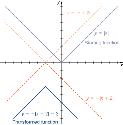
Figure $\PageIndex{14}$: The function $f(x)=−|x+2|−3$ can be viewed as a sequence of three transformations of the function $y=|x|$.

2. Starting with the graph of y=x√, reflect about the y-axis, stretch the graph vertically by a factor of 3, and move up 1 unit.

$imageedit_39_5995546184.png$

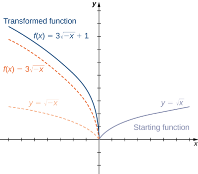
Figure $\PageIndex{15}$: The function $f(x)=\sqrt[3]{x}+1$can be viewed as a sequence of three transformations of the function $y=\sqrt{x}$.

Exercise $\PageIndex{7}$

Describe how the function $f(x)=−(x+1)^2−4$ can be graphed using the graph of $y=x^2$ and a sequence of transformations

Answer: Shift the graph $y=x^2$ to the left 1 unit, reflect about the $x$-axis, then shift down 4 units.

Key Concepts

The power function $f(x)=x^n$ is an even function if n is even and $n≠0$, and it is an odd function if $n$ is odd.
The root function $f(x)=x^{1/n}$ has the domain $[0,∞)$ if n is even and the domain $(−∞,∞)$ if $n$ is odd. If $n$ is odd, then $f(x)=x^{1/n}$ is an odd function.
The domain of the rational function $f(x)=p(x)/q(x)$, where $p(x)$ and $q(x)$ are polynomial functions, is the set of x such that $q(x)≠0$.
Functions that involve the basic operations of addition, subtraction, multiplication, division, and powers are algebraic functions.
Vertical and horizontal shifts, vertical and horizontal scalings, and reflections about the $x$- and $y$-axes are examples of transformations of functions.

Key Equations

Point-slope equation of a line

$y−y1=m(x−x_1)$

Slope-intercept form of a line

$y=mx+b$

Standard form of a line

$ax+by=c$

Polynomial function

$f(x)=a_n^{x^n}+a_{n−1}x^{n−1}+⋯+a_1x+a_0$

Glossary

algebraic function: a function involving any combination of only the basic operations of addition, subtraction, multiplication, division, powers, and roots applied to an input variable $x$

cubic function: a polynomial of degree 3; that is, a function of the form $f(x)=ax^3+bx^2+cx+d$, where $a≠0$

degree: for a polynomial function, the value of the largest exponent of any term

linear function: a function that can be written in the form $f(x)=mx+b$

mathematical model: A method of simulating real-life situations with mathematical equations

point-slope equation

equation of a linear function indicating its slope and a point on the graph of the function

polynomial function: a function of the form $f(x)=a_nx^n+a_{n−1}x^{n−1}+…+a_1x+a_0$

power function: a function of the form $f(x)=x^n$ for any positive integer $n≥1$

quadratic function: a polynomial of degree 2; that is, a function of the form $f(x)=ax^2+bx+c$ where $a≠0$

rational function: a function of the form $f(x)=p(x)/q(x)$, where $p(x)$ and $q(x)$ are polynomials

root function: a function of the form $f(x)=x^{1/n}$ for any integer $n≥2$

slope: the change in y for each unit change in x

slope-intercept form: equation of a linear function indicating its slope and y-intercept

transformation of a function

a shift, scaling, or reflection of a function

Contributors

Gilbert Strang (MIT) and Edwin “Jed” Herman (Harvey Mudd) with many contributing authors. This content by OpenStax is licensed with a CC-BY-SA-NC 4.0 license. Download for free at http://cnx.org.

Transformation of \(f (c>0)\)	Effect of the graph of \(f\)
\(f(x)+c\)	Vertical shift up \(c\) units
\(f(x)-c\)	Vertical shift down \(c\) units
\(f(x+c)\)	Shift left by \(c\) units
\(f(x-c)\)	Shift right by \(c\) units
\(cf(x)\)	Vertical stretch if \(c>1\); vertical compression if \(0<c<1\)
\(f(cx)\)	Horizontal stretch if \(0<c<1\); horizontal compression if \(c>1\)
\(-f(x)\)	Reflection about the \(x\)-axis
\(-f(x)\)	Reflection about the \(y\)-axis