
7.2: Modeling with Linear Functions


- Last updated
- Jan 11, 2022
- Save as PDF

( \newcommand{\kernel}{\mathrm{null}\,}\)
- Build linear models from verbal descriptions and two data points
- Solve a system of two linear equations using technology
- Construct a scatter plot to determine if there is a positive, negative, or no linear correlation
to apply mathematical modeling to solve real-world applications.
Emily is a college student who plans to spend a summer in Seattle. She has saved $3,500 for her trip and anticipates spending $400 each week on rent, food, and activities. How can we write a linear model to represent her situation? What would be the x-intercept, and what can she learn from it? To answer these and related questions, we can create a model using a linear function. Models such as this one can be extremely useful for analyzing relationships and making predictions based on those relationships. In this section, we will explore examples of linear function models.

Identifying Steps to Model and Solve Problems
When modeling scenarios with linear functions and solving problems involving quantities with a constant rate of change, we typically follow the same problem strategies that we would use for any type of function. Let’s briefly review them:
- Identify changing quantities, and then define descriptive variables to represent those quantities. When appropriate, sketch a picture or define a coordinate system.
- Carefully read the problem to identify important information. Look for information that provides values for the variables or values for parts of the functional model, such as slope and initial value.
- Carefully read the problem to determine what we are trying to find, identify, solve, or interpret.
- Identify a solution pathway from the provided information to what we are trying to find. Often this will involve checking and tracking units, building a table, or even finding a formula for the function being used to model the problem.
- When needed, write a formula for the function.
- Solve or evaluate the function using the formula.
- Reflect on whether your answer is reasonable for the given situation and whether it makes sense mathematically.
- Clearly convey your result using appropriate units, and answer in full sentences when necessary.
Building Linear Models
Now let’s take a look at the student in Seattle. In her situation, there are two changing quantities: time and money. The amount of money she has remaining while on vacation depends on how long she stays. We can use this information to define our variables, including units.
- Output: M, money remaining, in dollars
- Input: t, time, in weeks
So, the amount of money remaining depends on the number of weeks: M(t)
We can also identify the initial value and the rate of change.
- Initial Value: She saved $3,500, so $3,500 is the initial value for M.
- Rate of Change: She anticipates spending $400 each week, so –$400 per week is the rate of change, or slope.
Notice that the unit of dollars per week matches the unit of our output variable divided by our input variable. Also, because the slope is negative, the linear function is decreasing. This should make sense because she is spending money each week.
The rate of change is constant, so we can start with the linear model M(t)=mt+b. Then we can substitute the intercept and slope provided.

To find the x-intercept, we set the output to zero, and solve for the input.
0=−400t+3500t=3500400=8.75
The x-intercept is 8.75 weeks. Because this represents the input value when the output will be zero, we could say that Emily will have no money left after 8.75 weeks.
When modeling any real-life scenario with functions, there is typically a limited domain over which that model will be valid—almost no trend continues indefinitely. Here the domain refers to the number of weeks. In this case, it doesn’t make sense to talk about input values less than zero. A negative input value could refer to a number of weeks before she saved $3,500, but the scenario discussed poses the question once she saved $3,500 because this is when her trip and subsequent spending starts. It is also likely that this model is not valid after the x-intercept, unless Emily will use a credit card and goes into debt. The domain represents the set of input values, so the reasonable domain for this function is 0≤t≤8.75.
In the above example, we were given a written description of the situation. We followed the steps of modeling a problem to analyze the information. However, the information provided may not always be the same. Sometimes we might be provided with an intercept. Other times we might be provided with an output value. We must be careful to analyze the information we are given, and use it appropriately to build a linear model.
Using a Given Intercept to Build a Model
Some real-world problems provide the y-intercept, which is the constant or initial value. Once the y-intercept is known, the x-intercept can be calculated. Suppose, for example, that Hannah plans to pay off a no-interest loan from her parents. Her loan balance is $1,000. She plans to pay $250 per month until her balance is $0. The y-intercept is the initial amount of her debt, or $1,000. The rate of change, or slope, is -$250 per month. We can then use the slope-intercept form and the given information to develop a linear model.
f(x)=mx+b=−250x+1000
Now we can set the function equal to 0, and solve for x to find the x-intercept.
0=−250+10001000=250x4=xx=4
The x-intercept is the number of months it takes her to reach a balance of $0. The x-intercept is 4 months, so it will take Hannah four months to pay off her loan.
Using a Given Input and Output to Build a Model
Many real-world applications are not as direct as the ones we just considered. Instead they require us to identify some aspect of a linear function. We might sometimes instead be asked to evaluate the linear model at a given input or set the equation of the linear model equal to a specified output.
![]() Given a word problem that includes two pairs of input and output values, use the linear function to solve a problem.
Given a word problem that includes two pairs of input and output values, use the linear function to solve a problem.
- Identify the input and output values.
- Convert the data to two coordinate pairs.
- Find the slope.
- Write the linear model.
- Use the model to make a prediction by evaluating the function at a given x-value.
- Use the model to identify an x-value that results in a given y-value.
- Answer the question posed.
A town’s population has been growing linearly. In 2004 the population was 6,200. By 2009 the population had grown to 8,100. Assume this trend continues.
- Predict the population in 2013.
- Identify the year in which the population will reach 15,000.
Solution
The two changing quantities are the population size and time. While we could use the actual year value as the input quantity, doing so tends to lead to very cumbersome equations because the y-intercept would correspond to the year 0, more than 2000 years ago!
To make computation a little nicer, we will define our input as the number of years since 2004:
- Input: t, years since 2004
- Output: P(t), the town’s population
To predict the population in 2013 (t=9), we would first need an equation for the population. Likewise, to find when the population would reach 15,000, we would need to solve for the input that would provide an output of 15,000. To write an equation, we need the initial value and the rate of change, or slope.
To determine the rate of change, we will use the change in output per change in input.
m=change in outputchange in input
The problem gives us two input-output pairs. Converting them to match our defined variables, the year 2004 would correspond to t=0, giving the point (0,6200). Notice that through our clever choice of variable definition, we have “given” ourselves the y-intercept of the function. The year 2009 would correspond to t=5, giving the point (5,8100).
The two coordinate pairs are (0,6200) and (5,8100). Recall that we encountered examples in which we were provided two points earlier in the chapter. We can use these values to calculate the slope.
m=8100−62005−0=19005=380 people per year
We already know the y-intercept of the line, so we can immediately write the equation:
P(t)=380t+6200
To predict the population in 2013, we evaluate our function at t=9.
P(9)=380(9)+6,200=9,620
If the trend continues, our model predicts a population of 9,620 in 2013.
To find when the population will reach 15,000, we can set P(t)=15000 and solve for t.
15000=380t+62008800=380tt≈23.158
Our model predicts the population will reach 15,000 in a little more than 23 years after 2004, or somewhere around the year 2027.
A company sells doughnuts. They incur a fixed cost of $25,000 for rent, insurance, and other expenses. It costs $0.25 to produce each doughnut.
- Write a linear model to represent the cost C of the company as a function of x, the number of doughnuts produced.
- Find and interpret the y-intercept.
Solution
a. C(x)=0.25x+25,000 b. The y-intercept is (0,25,000). If the company does not produce a single doughnut, they still incur a cost of $25,000.
A city’s population has been growing linearly. In 2008, the population was 28,200. By 2012, the population was 36,800. Assume this trend continues.
- Predict the population in 2014.
- Identify the year in which the population will reach 54,000.
Solution
a. 41,100 b. 2020
Building Systems of Linear Models
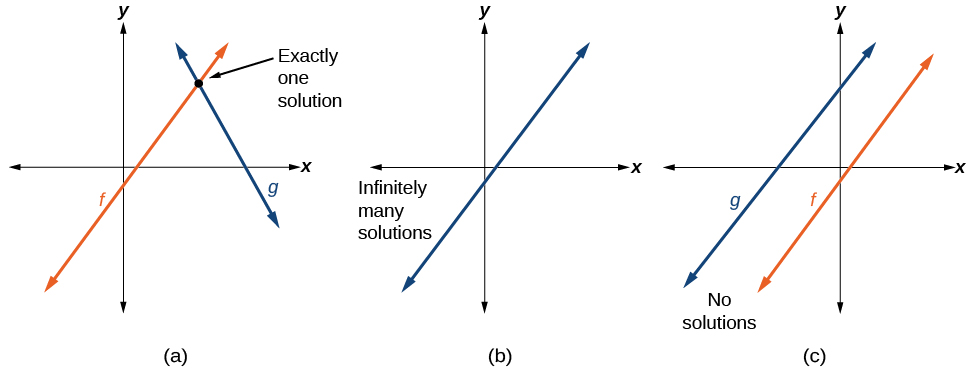
The previous section involved only one linear model. Oftentimes, real-world situations will include two or more linear functions which may be modeled with a system of linear equations. When solving a system of linear equations, we are looking for points the two lines have in common. Typically, there are three types of answers possible, as shown in Figure 7.2.6.
![]() Given a situation that represents a system of linear equations, write the system of equations and identify the solution.
Given a situation that represents a system of linear equations, write the system of equations and identify the solution.
- Identify the input and output of each linear model.
- Identify the slope and y-intercept of each linear model.
- Find the solution by setting the two linear functions equal to another and solving for x,or find the point of intersection on a graph (this is most easily done with technology such as desmos).
Jamal is choosing between two truck-rental companies. The first, Keep on Trucking, Inc., charges an up-front fee of $20, then 59 cents a mile[1]. The second, Move It Your Way, charges an up-front fee of $16, then 63 cents a mile. When will Keep on Trucking, Inc. be the better choice for Jamal?
Solution
The two important quantities in this problem are the cost and the number of miles driven. Because we have two companies to consider, we will define two functions.
- Input: d, distance driven in miles
- Outputs: K(d): cost, in dollars, for renting from Keep on Trucking
M(d): cost, in dollars, for renting from Move It Your Way
- Initial Value: Up-front fee: K(0)=20 and M(0)=16
- Rate of Change: K(d)=$0.59mile and P(d)=$0.63mile
A linear function is of the form f(x)=mx+b. Using the rates of change and initial charges, we can write the equations
K(d)=0.59d+20
M(d)=0.63d+16
Using these equations, we can determine when Keep on Trucking, Inc., will be the better choice. Because all we have to make that decision from is the costs, we are looking for when Move It Your Way, will cost less, or when K(d)<M(d). The solution pathway will lead us to find the equations for the two functions, find the intersection, and then see where the K(d) function is smaller.
These graphs are sketched in Figure 7.2.7, with K(d) in blue.
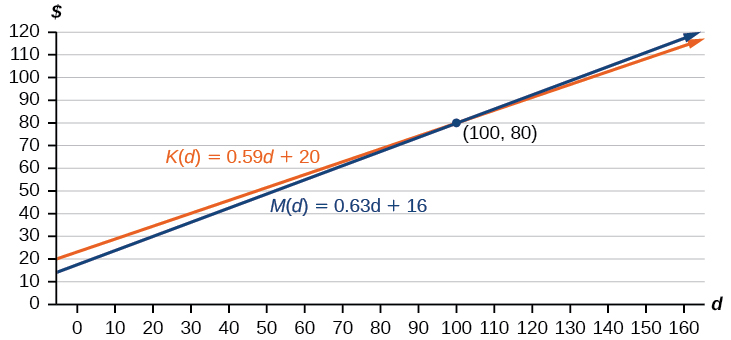
To find the intersection, we set the equations equal and solve:
K(d)=M(d)0.59d+20=0.63d+164=0.04d100=dd=100
This tells us that the cost from the two companies will be the same if 100 miles are driven. Either by looking at the graph, or noting that K(d) is growing at a slower rate, we can conclude that Keep on Trucking, Inc. will be the cheaper price when more than 100 miles are driven, that is d>100.
Please note this problem is easily solved by typing in the equations into desmos and clicking on the point of intersection to highlight the coordinates. You can see the result at https://www.desmos.com/calculator/hlnsxjksmy
Scatter Plots and Correlation
So far, we have been exploring linear relationships where we are given two data points which are used to construct the model. However, we will find that in many real-world applications that we have more than just two data points. In those cases, it's likely that the points don't all perfectly line up which will make constructing a linear model more difficult. It's important to first graph the points on a scatter plot to see if the data roughly follows a linear pattern, which is also known as a linear correlation. A correlation is simply a pattern that connects the input and output variables, and our goal is to investigate if the pattern is linear, and if it is, to eventually come up with an equation that expresses the correlation.
Let's start by exploring scatter plots with an example problem. Please remember that scatter plots are most easily constructed by using technology such as desmos.
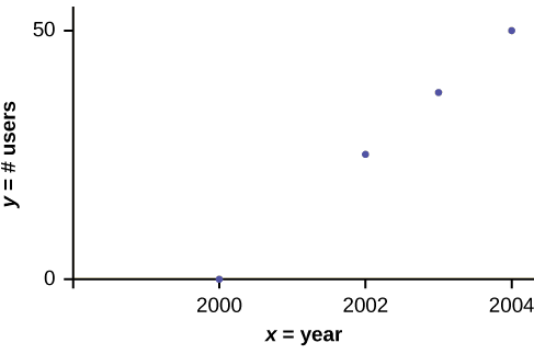
In Europe and Asia, m-commerce is popular. M-commerce users have special mobile phones that work like electronic wallets as well as provide phone and Internet services. Users can do everything from paying for parking to buying a TV set or soda from a machine to banking to checking sports scores on the Internet. For the years 2000 through 2004, was there a relationship between the year and the number of m-commerce users? Construct a scatter plot. Let x= the year and let y= the number of m-commerce users, in millions.
| x (year) | y (# of users) |
|---|---|
| 2000 | 0.5 |
| 2002 | 20.0 |
| 2003 | 33.0 |
| 2004 | 47.0 |
Go to desmos and create a table. From there, fill in the first column with the input values, and the second column with the associated output values. Make sure that the ordered pairs are still together and double-check that your table matches the given information! From there, the graph of the points will automatically generate.
Amelia plays basketball for her high school. She wants to improve to play at the college level. She notices that the number of points she scores in a game goes up in response to the number of hours she practices her jump shot each week. She records the following data:
| X (hours practicing jump shot) | Y (points scored in a game) |
|---|---|
| 5 | 15 |
| 7 | 22 |
| 9 | 28 |
| 10 | 31 |
| 11 | 33 |
| 12 | 36 |
Construct a scatter plot and state if what Amelia thinks appears to be true.
- Answer
-
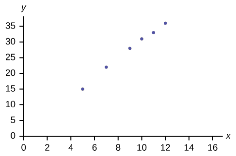
Figure 7.2.6
Yes, Amelia’s assumption appears to be correct. The number of points Amelia scores per game goes up when she practices her jump shot more.
A scatter plot shows the direction of a relationship between the variables. A clear direction happens when there is either:
- High values of one variable occurring with high values of the other variable or low values of one variable occurring with low values of the other variable.
- High values of one variable occurring with low values of the other variable.
You can determine the strength of the relationship by looking at the scatter plot and seeing how close the points are to a line, a power function, an exponential function, or to some other type of function. For a linear relationship there is an exception. Consider a scatter plot where all the points fall on a horizontal line providing a "perfect fit." The horizontal line would in fact show no relationship.
When you look at a scatter plot, you want to notice the overall pattern and any deviations from the pattern. The following scatterplot examples illustrate these concepts.
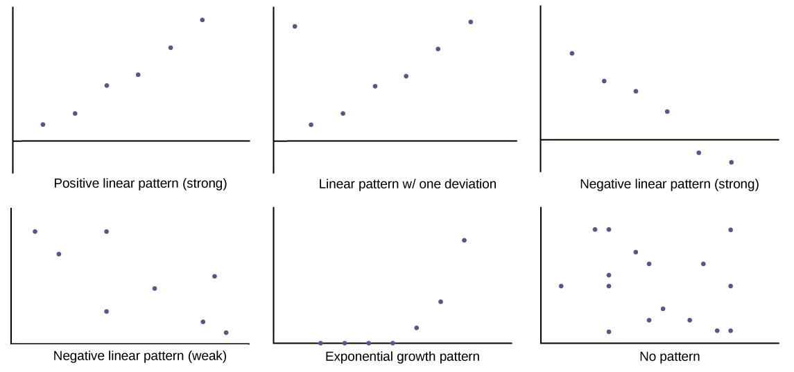
In the next section, we are interested in scatter plots that show a linear pattern. Linear patterns are quite common. The linear relationship is strong if the points are close to a straight line, except in the case of a horizontal line where there is no relationship. If we think that the points show a linear relationship, we would like to draw a line on the scatter plot. This line can be calculated through a process called linear regression. However, we only calculate a regression line if one of the variables helps to explain or predict the other variable. If x is the independent variable and y the dependent variable, then we can use a regression line to predict y for a given value of x