1.1: The Pythagorean Theorem

Learning Objectives

• Use the Pythagorean Theorem to determine if a triangle is a right triangle.
• Use the Pythagorean Theorem to determine the length of one side of a right triangle.
• Use the distance formula to determine the distance between two points on the coordinate plane.

Recall the following definitions from elementary geometry:

1. An angle is acute if it is between \(0°\) and \(90°\).
2. An angle is a right angle if it equals \(90°\).
3. An angle is obtuse if it is between \(90°\) and \(180°\).
4. An angle is a straight angle if it equals \(180°\).

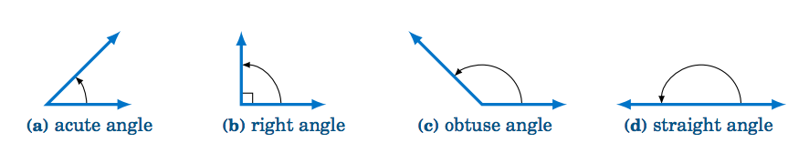
Figure 1.1.1 Types of angles

In elementary geometry, angles are always considered to be positive and not larger than \(360^\circ \). For now we will only consider such angles. The following definitions will be used throughout the text:

1. Two acute angles are complementary if their sum equals \(90^◦\). In other words, if \(0^◦ ≤ ∠ A , ∠B ≤ 90^◦ \text{ then }∠ A \text{ and }∠B\) are complementary if \(∠ A +∠B = 90^◦\).
2. Two angles between \(0^◦ \text{ and }180^◦\) are supplementary if their sum equals \(180^◦\). In other words, if \(0^◦ ≤ ∠ A , ∠B ≤ 180^◦ \text{ then }∠ A \text{ and }∠B\) are supplementary if \(∠ A +∠B = 180^◦\).
3. Two angles between \(0^◦ \text{ and }360^◦\) are conjugate (or explementary) if their sum equals \(360^◦\). In other words, if \(0^◦ ≤ ∠ A , ∠B ≤ 360^◦ \text{ then }∠ A \text{ and }∠B\text{ are conjugate if }∠ A+∠B = 360^◦\).

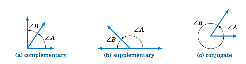
Figure 1.1.2 Types of pairs of angles

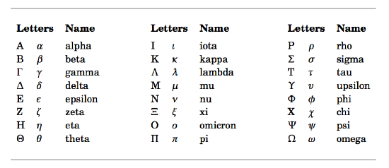
Instead of using the angle notation \(∠ A\) to denote an angle, we will sometimes use just a capital letter by itself (e.g. \(A, B, C\)) or a lowercase variable name (e.g. \(x, y, t\)). It is also common to use letters (either uppercase or lowercase) from the Greek alphabet, shown in the table below, to represent angles:

Table 1.1 The Greek alphabet

In elementary geometry you learned that the sum of the angles in a triangle equals \(180^◦\), and that an isosceles triangle is a triangle with two sides of equal length. Recall that in a right triangle one of the angles is a right angle. Thus, in a right triangle one of the angles is \(90^◦\) and the other two angles are acute angles whose sum is \(90^◦\) (i.e. the other two angles are complementary angles).

\[\nonumber α + 3α + α = 180^◦ ⇒ 5α = 180^◦ ⇒ α = 36^◦ ⇒ \fbox{\(X = 36^◦ ,\, Y = 3×36^◦ = 108^◦ ,\, Z = 36^◦\)}\]

QED

Figure 1.1.3

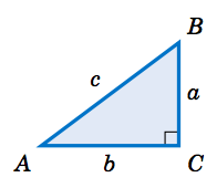
By knowing the lengths of two sides of a right triangle, the length of the third side can be determined by using the Pythagorean Theorem:

\(a^2+b^2=c^2\)

The square of the length of the hypotenuse of a right triangle is equal to the sum of the squares of the lengths of its legs.

Figure 1.1.4 Similar triangles \(△ ABC, △CBD, △ ACD\)

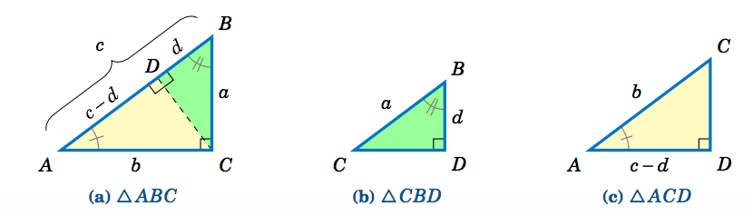
Recall that triangles are similar if their corresponding angles are equal, and that similarity implies that corresponding sides are proportional. Thus, since \(\triangle\,ABC \) is similar to \(\triangle\,CBD \), by proportionality of corresponding sides we see that

\[\nonumber \overline{AB}~\text{is to}~\overline{CB}~\text{(hypotenuses)}\text{ as }
\overline{BC}~\text{is to}~\overline{BD}~\text{(vertical legs)}
\quad\Rightarrow\quad \frac{c}{a} ~=~ \frac{a}{d} \quad\Rightarrow\quad cd ~=~ a^2 ~.\]

Since \(\triangle\,ABC \) is similar to \(\triangle\,ACD \), comparing horizontal legs and hypotenuses gives

\[\nonumber \frac{b}{c-d} ~=~ \frac{c}{b} \quad\Rightarrow\quad b^2 ~=~ c^2 ~-~ cd ~=~ c ^2 ~-~ a^2
\quad\Rightarrow\quad a^2 ~+~ b^2 ~=~ c^2 ~. \textbf{QED}\]

Note: The symbols \(\perp\) and \(\sim\) denote perpendicularity and similarity, respectively. For example, in the above proof we had \(\,\overline{CD} \perp \overline{AB}\, \) and \(\,\triangle\,ABC \sim \triangle\,CBD \sim \triangle\,ACD \).

For triangle \(\triangle\,ABC \), the Pythagorean Theorem says that

\[\nonumber a^2 ~+~ 4^2 ~=~ 5^2 \quad\Rightarrow\quad a^2 ~=~ 25 ~-~ 16 ~=~ 9 \quad\Rightarrow\quad
\fbox{\(a ~=~ 3\)} ~.\]

For triangle \(\triangle\,DEF \), the Pythagorean Theorem says that

\[\nonumber e^2 ~+~ 1^2 ~=~ 2^2 \quad\Rightarrow\quad e^2 ~=~ 4 ~-~ 1 ~=~ 3 \quad\Rightarrow\quad
\fbox{$e ~=~ \sqrt{3}$} ~.\]

For triangle \(\triangle\,XYZ \), the Pythagorean Theorem says that

\[\nonumber 1^2 ~+~ 1^2 ~=~ z^2 \quad\Rightarrow\quad z^2 ~=~ 2 \quad\Rightarrow\quad
\fbox{$z ~=~ \sqrt{2}$} ~.\]

Let \(h \) be the height at which the ladder touches the wall. We can assume that the ground makes a right angle with the wall, as in the picture on the right. Then we see that the ladder, ground, and wall form a right triangle with a hypotenuse of length 17 ft (the length of the ladder) and legs with lengths 8 ft and \(h \) ft. So by the Pythagorean Theorem, we have

\[\nonumber h^2 ~+~ 8^2 ~=~ 17^2 \quad\Rightarrow\quad h^2 ~=~ 289 ~-~ 64 ~=~ 225 \quad\Rightarrow\quad
\fbox{$h ~=~ 15 ~\text{ft}$} ~.\]

Determining the Distance Using the Pythagorean Theorem

You can use the Pythagorean Theorem is to find the distance between two points.

Consider the points (-1, 6) and (5, -3). If we plot these points on a grid and connect them, they make a diagonal line. Draw a vertical line down from (-1, 6) and a horizontal line to the left of (5, -3) to make a right triangle.

Figure \(\PageIndex{5}\)

Now we can find the distance between these two points by using the vertical and horizontal distances that we determined from the graph.

\(\begin{aligned} 9^2+(−6)^2 &=d^2 \\ 81+36 &=d^2 \\ 117 &=d^2\\ \sqrt{117}&=d \\ 3\sqrt{13}&=d\end{aligned}\)

Notice, that the x−values were subtracted from each other to find the horizontal distance and the y−values were subtracted from each other to find the vertical distance. If this process is generalized for two points \((x_1, y_1)\)and \((x_2, y_2)\), the Distance Formula is derived.

\((x_1−x_2)^2+(y_1−y_2)^2=d^2\)

Figure \(\PageIndex{6}\)

This is the Pythagorean Theorem with the vertical and horizontal differences between \((x_1, y_1)\) and \((x_2, y_2)\). Taking the square root of both sides will solve the right hand side for d, the distance.

\(\sqrt{(x_1−x_2)^2+(y_1−y_2)^2}=d\)

This is the Distance Formula.

Contributors and Attributions

• Michael Corral (Schoolcraft College). The content of this page is distributed under the terms of the GNU Free Documentation License, Version 1.2.