1.6: Operations with Matrices

In the previous section we saw the important connection between linear functions and matrices. In this section we will discuss various operations on matrices which we will find useful in our later work with linear functions.

The algebra of matrices

If \(M\) is an \(n \times m\) matrix with \(a_{i j}\) in the \(i\)th row and \(j\)th column, \(i=1,2, \ldots, n, j= 1,2, \ldots, m\), then we will write \(M=\left[a_{i j}\right]\). With this notation the definitions of addition, subtraction, and scalar multiplication for matrices are straightforward.

Definition \(\PageIndex{1}\)

Suppose \(M=\left[a_{i j}\right]\) and \(N=\left[b_{i j}\right]\) are \(n \times m\) matrices and \(c\) is a real number. Then we define

\[ M+N=\left[a_{i j}+b_{i j}\right],\]

\[M-N=\left[a_{i j}-b_{i j}\right],\]

and

\[c M=\left[c a_{i j}\right] .\]

In other words, we define addition, subtraction, and scalar multiplication for matrices by performing these operations on the individual elements of the matrices, in a manner similar to the way we perform these operations on vectors.

Example \(\PageIndex{1}\)

If

\[ M=\left[\begin{array}{rrr}
1 & 2 & 3 \\
-5 & 3 & -1
\end{array}\right] \nonumber \]

and

\[N=\left[\begin{array}{rrr}
3 & 1 & 4 \\
1 & -3 & 2
\end{array}\right], \nonumber \]

then, for example,

\[\begin{aligned}
&M+N=\left[\begin{array}{rrr}
1+3 & 2+1 & 3+4 \\
-5+1 & 3-3 & -1+2
\end{array}\right]=\left[\begin{array}{rrr}
4 & 3 & 7 \\
-4 & 0 & 1
\end{array}\right], \\
&M-N=\left[\begin{array}{rrr}
1-3 & 2-1 & 3-4 \\
-5-1 & 3+3 & -1-2
\end{array}\right]=\left[\begin{array}{lll}
-2 & 1 & -1 \\
-6 & 6 & -3
\end{array}\right],
\end{aligned} \nonumber \]

and

\[3 M=\left[\begin{array}{rrr}
3 & 6 & 9 \\
-15 & 9 & -2
\end{array}\right]. \nonumber \]

These operations have natural interpretations in terms of linear functions. Suppose \(L: \mathbb{R}^{m} \rightarrow \mathbb{R}^{n}\) and \(K: \mathbb{R}^{m} \rightarrow \mathbb{R}^{n}\) are linear with \(L(\mathbf{x})=M \mathbf{x}\) and \(K(\mathbf{x})=N \mathbf{x}\) for \(n \times m\) matrices \(M\) and \(N\). If we define \(L+K: \mathbb{R}^{n} \rightarrow \mathbb{R}^{m}\) by

\[ (L+K)(\mathbf{x})=L(\mathbf{x})+K(\mathbf{x}) ,\]

then

\[ (L+K)\left(\mathbf{e}_{j}\right)=L\left(\mathbf{e}_{j}\right)+K\left(\mathbf{e}_{j}\right) \]

for \(j=1,2, \ldots, m\). Hence the \(j\)th column of the matrix which represents \(L+K\) is the sum of the \(j\)th columns of \(M\) and \(N\). In other words,

\[ (L+K)(\mathbf{x})=(M+N) \mathbf{x}\]

for all \(\mathbf{x}\) in \(\mathbb{R}^{m}\). Similarly, if we define \(L-K: \mathbb{R}^{m} \rightarrow \mathbb{R}^{n}\) by

\[ (L-K)(\mathbf{x})=L(\mathbf{x})-K(\mathbf{x}) ,\]

then

\[(L-K)(\mathbf{x})=(M-N) \mathbf{x} .\]

If, for any scalar \(c\), we define \(c L: \mathbb{R}^{m} \rightarrow \mathbb{R}^{n}\) by

\[ c L(\mathbf{x})=c(L(\mathbf{x})) ,\]

then

\[ c L\left(\mathbf{e}_{j}\right)=c\left(L\left(\mathbf{e}_{j}\right)\right) \]

for \(j=1,2, \ldots, m\). Hence the \(j\)th column of the matrix which represents \(cL\) is the scalar \(c\) times the \(j\)th column of \(M\). That is,

\[ c L(\mathbf{x})=(c M) \mathbf{x} \]

for all \(\mathbf{x}\) in \(\mathbb{R}^{m}\). In short, the operations of addition, subtraction, and scalar multiplication for matrices corresponds in a natural way with the operations of addition, subtraction, and scalar multiplication for linear functions.

Now consider the case where \(L: \mathbb{R}^{m} \rightarrow \mathbb{R}^{p}\) and \(K: \mathbb{R}^{p} \rightarrow \mathbb{R}^{n}\) are linear functions. Let \(M\) be the \(p \times m\) matrix such that \(L(\mathbf{x})=M \mathbf{x}\) for all \(\mathbf{x}\) in \(\mathbb{R}^{m}\) and let \(N\) be the \(n \times p\) matrix such that \(K(\mathbf{x})=N \mathbf{x}\) for all \(\mathbf{x}\) in \(\mathbb{R}^{p}\). Since for any \(\mathbf{x}\) in \(\mathbb{R}^{m}\), \(L(\mathbf{x})\) is in \(\mathbb{R}^{p}\), we can form \(K \circ L: \mathbb{R}^{m} \rightarrow \mathbb{R}^{n}\), the composition of \(K\) with \(L\), defined by

\[ K \circ L(\mathbf{x})=K(L(\mathbf{x})). \]

Now

\[ K(L(\mathbf{x}))=N(M \mathbf{x}) ,\]

so it would be natural to define \(NM\), the product of the matrices \(N\) and \(M\), to be the matrix of \(K \circ L\), in which case we would have

\[ N(M \mathbf{x})=(N M) \mathbf{x}.\]

Thus we want the \(j\)th column of \(NM\), \(j=1,2, \ldots, m\), to be

\[K \circ L\left(\mathbf{e}_{j}\right)=N\left(L\left(\mathbf{e}_{j}\right)\right),\]

which is just the dot product of \(L\left(\mathbf{e}_{j}\right)\) with the rows of \(N\). But \(L\left(\mathbf{e}_{j}\right)\) is the \(j\)th column of \(M\), so the \(j\)th column of \(NM\) is formed by taking the dot product of the \(j\)th column of \(M\) with the rows of \(N\). In other words, the entry in the \(i\)th row and \(j\)th column of \(NM\) is the dot product of the \(i\)th row of \(N\) with the \(j\)th column of \(M\). We write this out explicitly in the following definition.

Definition \(\PageIndex{2}\)

If \(N=\left[a_{i j}\right]\) is an \(n \times p\) matrix and \(M=\left[b_{i j}\right]\) is a \(p \times m\) matrix, then we define the product of \(N\) and \(M\) to be the \(n \times m\) matrix \(N M=\left[c_{i j}\right]\), where

\[ c_{i j}=\sum_{k=1}^{p} a_{i k} b_{k j} , \]

\(i=1,2, \ldots, n \text { and } j=1,2, \ldots, m . \)

Note that \(NM\) is an \(n \times m\) matrix since \(K \circ L: \mathbb{R}^{m} \rightarrow \mathbb{R}^{n}\). Moreover, the product \(NM\) of two matrices \(N\) and \(M\) is defined only when the number of columns of \(N\) is equal to the number of rows of \(M\).

Example \(\PageIndex{2}\)

If

\[ N=\left[\begin{array}{rr}
1 & 2 \\
-1 & 3 \\
2 & -2
\end{array}\right] \nonumber \]

and

\[ M=\left[\begin{array}{rrrr}
2 & -2 & 1 & 3 \\
1 & 2 & -1 & -2
\end{array}\right] , \nonumber \]

then

\begin{aligned}
N M &=\left[\begin{array}{rr}
1 & 2 \\
-1 & 3 \\
2 & -2
\end{array}\right]\left[\begin{array}{rrrr}
2 & -2 & 1 & 3 \\
1 & 2 & -1 & -2
\end{array}\right] \\
&=\left[\begin{array}{rrrr}
2+2 & -2+4 & 1-2 & 3-4 \\
-2+3 & 2+6 & -1-3 & -3-6 \\
4-2 & -4-4 & 2+2 & 6+4
\end{array}\right] \\
&=\left[\begin{array}{rrrr}
4 & 2 & -1 & -1 \\
1 & 8 & -4 & -9 \\
2 & -8 & 4 & 10
\end{array}\right] .
\end{aligned}

Note that \(N\) is \(3 \times 2\), \(M\) is \(2 \times 4\), and \(NM\) is \(3 \times 4\). Also, note that it is not possible to form the product in the other order.

Example \(\PageIndex{3}\)

Let \(L: \mathbb{R}^{2} \rightarrow \mathbb{R}^{3}\) be the linear function defined by

\[ L(x, y)=(3 x-2 y, x+y, 4 y) \nonumber \]

and let \(K: \mathbb{R}^{3} \rightarrow \mathbb{R}^{2}\) be the linear function defined by

\[ K(x, y, z)=(2 x-y+z, x-y-z). \nonumber\]

Then the matrix for \(L\) is

\[ M=\left[\begin{array}{rr}
3 & -2 \\
1 & 1 \\
0 & 4
\end{array}\right] , \nonumber \]

the matrix for \(K\) is

\[ N=\left[\begin{array}{rrr}
2 & -1 & 1 \\
1 & -1 & -1
\end{array}\right] , \nonumber \]

and the matrix for \(K \circ L: \mathbb{R}^{2} \rightarrow \mathbb{R}^{2}\) is

\[ N M=\left[\begin{array}{rrr}
2 & -1 & 1 \\
1 & -1 & -1
\end{array}\right]\left[\begin{array}{rr}
3 & -2 \\
1 & 1 \\
0 & 4
\end{array}\right]=\left[\begin{array}{ll}
6-1+0 & -4-1+4 \\
3-1+0 & -2-1-4
\end{array}\right]=\left[\begin{array}{ll}
5 & -1 \\
2 & -7
\end{array}\right] . \nonumber \]

In other words,

\[ K \circ L(x, y)=\left[\begin{array}{ll}
5 & -1 \\
2 & -7
\end{array}\right]\left[\begin{array}{l}
x \\
y
\end{array}\right]=\left[\begin{array}{c}
5 x-y \\
2 x-7 y
\end{array}\right] . \nonumber \]

Note that it in this case it is possible to form the composition in the other order. The matrix for \(L \circ K: \mathbb{R}^{3} \rightarrow \mathbb{R}^{3}\) is

\[ M N=\left[\begin{array}{rr}
3 & -2 \\
1 & 1 \\
0 & 4
\end{array}\right]\left[\begin{array}{rrr}
2 & -1 & 1 \\
1 & -1 & -1
\end{array}\right]=\left[\begin{array}{rrr}
6-2 & -3+2 & 3+2 \\
2+1 & -1-1 & 1-1 \\
0+4 & 0-4 & 0-4
\end{array}\right]=\left[\begin{array}{rrr}
4 & -1 & 5 \\
3 & -2 & 0 \\
4 & -4 & -4
\end{array}\right] , \nonumber \]

and so

\[ L \circ K(x, y, z)=\left[\begin{array}{rrr}
4 & -1 & 5 \\
3 & -2 & 0 \\
4 & -4 & -4
\end{array}\right]\left[\begin{array}{l}
x \\
y \\
z
\end{array}\right]=\left[\begin{array}{c}
4 x-y+5 z \\
3 x-2 y \\
4 x-4 y-4 z
\end{array}\right] . \nonumber \]

In particular, note that not only is \(N M \neq M N\), but in fact \(NM\) and \(MN\) are not even the same size.

Determinants

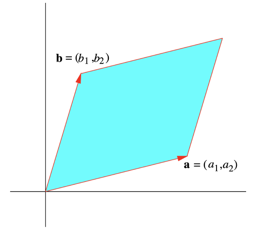
The notion of the determinant of a matrix is closely related to the idea of area and volume. To begin our definition, consider the \(2 \times 2\) matrix

\[ M=\left[\begin{array}{ll}
a_{1} & a_{2} \\
b_{1} & b_{2}
\end{array}\right] \nonumber \]

Figure \(\PageIndex{1}\): A parallelogram in \(\mathbb{R}^{2}\) with adjacent sides \(\mathbf{a}\) and \(\mathbf{b}\)

and let \(\mathbf{a}=\left(a_{1}, a_{2}\right)\) and \(\mathbf{b}=\left(b_{1}, b_{2}\right)\). If \(P\) is the parallelogram which has \(\mathbf{a}\) and \(\mathbf{b}\) for adjacent sides and \(A\) is the area of \(P\) (see Figure 1.6.1), then we saw in Section 1.3 that

\[ A=\left\|\left(a_{1}, a_{2}, 0\right) \times\left(b_{1}, b_{2}, 0\right)\right\|=\|\left(0,0, a_{1} b_{2}-a_{2} b_{1} \|=\left|a_{1} b_{2}-a_{2} b_{1}\right|\right. . \]

This motivates the following definition.

Definition \(\PageIndex{3}\)

Given a \(2 \times 2\) matrix

\[M=\left[\begin{array}{ll}
a_{1} & a_{2} \\
b_{1} & b_{2}
\end{array}\right], \nonumber \]

the determinant of \(M\), denoted det(\(M\)), is

\[ \operatorname{det}(M)=a_{1} b_{2}-a_{2} b_{1} . \label{1.6.18} \]

Hence we have \(A=|\operatorname{det}(M)|\). In words, for a \(2 \times 2\) matrix \(M\), the absolute value of the determinant of \(M\) equals the area of the parallelogram which has the rows of \(M\) for adjacent sides.

Example \(\PageIndex{4}\)

We have

\[ \operatorname{det}\left[\begin{array}{rr}
1 & 3 \\
-4 & 5
\end{array}\right]=(1)(5)-(3)(-4)=5+12=17. \nonumber \]

Now consider a \(3 \times 3\) matrix

\[ M=\left[\begin{array}{lll}
a_{1} & a_{2} & a_{3} \\
b_{1} & b_{2} & b_{3} \\
c_{1} & c_{2} & c_{3}
\end{array}\right] \nonumber \]

and let \(\mathbf{a}=\left(a_{1}, a_{2}, a_{3}\right)\), \(\mathbf{b}=\left(b_{1}, b_{2}, b_{3}\right)\), and \(\mathbf{c}=\left(c_{1}, c_{2}, c_{3}\right)\). If \(V\) is the volume of the parallelepiped \(P\) with adjacent edges \(\mathbf{a}\), \(\mathbf{b}\), and \(\mathbf{c}\), then, again from Section 1.3,

\[ \begin{align}
V &=|\mathbf{a} \cdot(\mathbf{b} \times \mathbf{c})| \nonumber \\
&=\left|a_{1}\left(b_{2} c_{3}-b_{3} c_{2}\right)+a_{2}\left(b_{3} c_{1}-b_{1} c_{3}\right)+a_{3}\left(b_{1} c_{2}-b_{2} c_{1}\right)\right| \nonumber \\
&=\left|a_{1} \operatorname{det}\left[\begin{array}{ll}
b_{2} & b_{3} \nonumber \\
c_{2} & c_{3}
\end{array}\right]-a_{2} \operatorname{det}\left[\begin{array}{ll}
b_{1} & b_{3} \nonumber \\
c_{1} & c_{3}
\end{array}\right]+a_{3} \operatorname{det}\left[\begin{array}{ll}
b_{1} & b_{2} \nonumber \\
c_{1} & c_{2}
\end{array}\right]\right| . \label{}
\end{align} \]

Definition \(\PageIndex{4}\)

Given a \(3 \times 3\) matrix

\[ M=\left[\begin{array}{lll}
a_{1} & a_{2} & a_{3} \\
b_{1} & b_{2} & b_{3} \\
c_{1} & c_{2} & c_{3}
\end{array}\right] , \nonumber \]

the determinant of \(M\), denoted det(\(M\)), is

\[ \operatorname{det}(M)=a_{1} \operatorname{det}\left[\begin{array}{ll}
b_{2} & b_{3} \\
c_{2} & c_{3}
\end{array}\right]-a_{2} \operatorname{det}\left[\begin{array}{ll}
b_{1} & b_{3} \\
c_{1} & c_{3}
\end{array}\right]+a_{3} \operatorname{det}\left[\begin{array}{ll}
b_{1} & b_{2} \\
c_{1} & c_{2}
\end{array}\right] . \label{1.6.20}\]

Similar to the \(2 \times 2\) case, we have \(V=|\operatorname{det}(M)|\).

Example \(\PageIndex{5}\)

We have

\begin{aligned}
\operatorname{det}\left[\begin{array}{llr}
2 & 3 & 9 \\
2 & 1 & -4 \\
5 & 1 & -1
\end{array}\right] &=2 \operatorname{det}\left[\begin{array}{cc}
1 & -4 \\
1 & -1
\end{array}\right]-3 \operatorname{det}\left[\begin{array}{cc}
2 & -4 \\
5 & -1
\end{array}\right]+9 \operatorname{det}\left[\begin{array}{cc}
2 & 1 \\
5 & 1
\end{array}\right] \\
&=2(-1+4)-3(-2+20)+9(2-5) \\
&=6-54-27 \\
&=-75 .
\end{aligned}

Given an \(n \times n \) matrix \(M=\left[a_{i j}\right]\), let \(M_{i j}\) be the \((n-1) \times(n-1)\) matrix obtained by deleting the \(i\)th row and \(j\)th column of \(M\). If for \(n=1\) we first define \(\operatorname{det}(M)=a_{11}\) (that is, the determinant of a \(1 \times 1 \) matrix is just the value of its single entry), then we could express, for \(n=2\), the definition of a the determinant of a \(2 \times 2 \) matrix given in (\(\ref{1.6.18}\)) in the form

\[ \operatorname{det}(M)=a_{11} \operatorname{det}\left(M_{11}\right)-a_{12} \operatorname{det}\left(M_{12}\right)=a_{11} a_{22}-a_{12} a_{21}. \]

Similarly, with \(n=3\), we could express the definition of the determinant of \(M\) given in (\(\ref{1.6.20}\)) in the form

\[ \operatorname{det}(M)=a_{11} \operatorname{det}\left(M_{11}\right)-a_{12} \operatorname{det}\left(M_{12}\right)+a_{13} \operatorname{det}\left(M_{13}\right). \]

Following this pattern, we may form a recursive definition for the determinant of an \(n \times n\) matrix.

Definition \(\PageIndex{5}\)

Suppose \(M=\left[a_{i j}\right]\) is an \(n \times n\) matrix and let \(M_{i j}\) be the \((n-1) \times(n-1)\) matrix obtained by deleting the \(i\)th row and \(j\)th column of \(M\), \(i=1,2, \ldots, n\) and \(j=1,2, \ldots, n\). For \(n=1\), we define the determinant of \(M\), denoted \(\operatorname{det}(M)\), by

\[ \operatorname{det}(M)=a_{11} \]

For \(n > 1\), we define the determinant of \(M\), denoted \(\operatorname{det}(M)\), by

\[ \begin{align}
\operatorname{det}(M) &=a_{11} \operatorname{det}\left(M_{11}\right)-a_{12} \operatorname{det}\left(M_{12}\right)+\cdots+(-1)^{1+n} a_{1 n} \operatorname{det}\left(M_{1 n}\right) \nonumber \\
&=\sum_{j=1}^{n}(-1)^{1+j} a_{1 j} \operatorname{det}\left(M_{1 j}\right). \label{1.6.24}
\end{align} \]

We call the definition recursive because we have defined the determinant of an \(n \times n\) matrix in terms of the determinants of \((n-1) \times(n-1)\) matrices, which in turn are defined in terms of the determinants of \((n-2) \times(n-2)\) matrices, and so on, until we have reduced the problem to computing the determinants of \(1 \times 1\) matrices.

Example \(\PageIndex{6}\)

For an example of the determinant of a \(4 \times 4\) matrix, we have

\begin{aligned}
\operatorname{det}\left[\begin{array}{rrrr}
2 & 1 & 3 & 2 \\
2 & 1 & 4 & 1 \\
-2 & 3 & -1 & 2 \\
1 & 2 & 1 & 1
\end{array}\right]=2 & \operatorname{det}\left[\begin{array}{rrr}
1 & 4 & 1 \\
3 & -1 & 2 \\
2 & 1 & 1
\end{array}\right]-\operatorname{det}\left[\begin{array}{rrr}
2 & 4 & 1 \\
-2 & -1 & 2 \\
1 & 11 & 1
\end{array}\right] \\
&+3 \operatorname{det}\left[\begin{array}{rrr}
2 & 1 & 1 \\
-2 & 3 & 2 \\
1 & 2 & 1
\end{array}\right]-2 \operatorname{det}\left[\begin{array}{rrr}
2 & 1 & 4 \\
-2 & 3 & -1 \\
1 & 2 & 1
\end{array}\right] \\
=& 2((-1-2)-4(3-4)+(3+2))-(2(-1-2)\\
&\quad-4(-2-2)+(-2+1))+3(2(3-4)-(-2-2)\\
&+(-4-3))-2(2(3+2)-(-2+1)+4(-4-3)) \\
=& 2(-3+4+5)-(-6+16-1)+3(-2+4-7) \\
& \quad-2(10+1-28) \\
=& 12-9-15+34 \\
=& 22 .
\end{aligned}

The next theorem states that there is nothing special about using the first row of the matrix in the expansion of the determinant specified in (\(\ref{1.6.24}\)), nor is there anything special about expanding along a row instead of a column. The practical effect is that we may compute the determinant of a given matrix expanding along whichever row or column is most convenient. The proof of this theorem would take us too far afield at this point, so we will omit it (but you will be asked to verify the theorem for the special cases \(n=2\) and \(n=3\) in Exercise 10).

Theorem \(\PageIndex{1}\)

Let \(M=\left[a_{i j}\right]\) be an \(n \times n\) matrix and let \(M_{i j}\) be the \((n-1) \times(n-1)\) matrix obtained by deleting the \(i\)th row and \(j\)th column of \(M\). Then for any \(i=1,2, \ldots, n\),

\[ \operatorname{det}(M)=\sum_{j=1}^{n}(-1)^{i+j} a_{i j} \operatorname{det}\left(M_{i j}\right), \]

and for any \(j=1,2, \ldots, n\),

\[ \operatorname{det}(M)=\sum_{i=1}^{n}(-1)^{i+j} a_{i j} \operatorname{det}\left(M_{i j}\right), \label{1.6.26} \]

Example \(\PageIndex{7}\)

The simplest way to compute the determinant of the matrix

\[ M=\left[\begin{array}{rrr}
4 & 0 & 3 \\
2 & 3 & 1 \\
-3 & 0 & -2
\end{array}\right] \nonumber \]

is to expand along the second column. Namely,

\begin{aligned}
\operatorname{det}(M)=&(-1)^{1+2}(0) \operatorname{det}\left[\begin{array}{rr}
2 & 1 \\
-3 & -2
\end{array}\right]+(-1)^{2+2}(3) \operatorname{det}\left[\begin{array}{rr}
4 & 3 \\
-3 & -2
\end{array}\right] \\
&+(-1)^{3+2}(0) \operatorname{det}\left[\begin{array}{ll}
4 & 3 \\
2 & 1
\end{array}\right] \\
=& 3(-8+9) \\
=& 3 .
\end{aligned}

You should verify that expanding along the first row, as we did in the definition of the determinant, gives the same result.

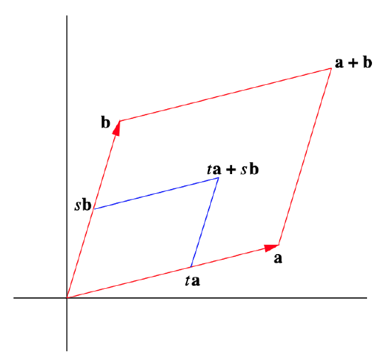
In order to return to the problem of computing volumes, we need to define a parallelepiped in \(\mathbb{R}^{n}\). First note that if \(P\) is a parallelogram in \(\mathbb{R}^{2}\) with adjacent sides given by the vectors \(\mathbf{a}\) and \(\mathbf{b}\), then

\[ P=\{\mathbf{y}: \mathbf{y}=t \mathbf{a}+s \mathbf{b}, 0 \leq t \leq 1,0 \leq s \leq 1\}. \]

That is, for \(0 \leq t \leq 1\), \(\text { ta }\) is a point between \(\mathbf{0}\) and \(\mathbf{a}\), and for \(0 \leq s \leq 1\), \(s \mathbf{b}\) is a point between \(\mathbf{0}\) and \(\mathbf{b}\); hence \(t \mathbf{a}+s \mathbf{b}\) is a point in the parallelogram \(P\). Moreover, every point in \(P\) may be expressed in this form. See Figure 1.6.2. The following definition generalizes this characterization of parallelograms.

Figure \(\PageIndex{2}\): A parallelogram in \(\mathbb{R}^{2}\) with adjacent sides \(\mathbf{a}\) and \(\mathbf{b}\)

Definition \(\PageIndex{6}\)

Let \(\mathbf{a}_{1}, \mathbf{a}_{2}, \ldots, \mathbf{a}_{n}\) be linearly independent vectors in \(\mathbb{R}^{n}\). We call

\[ P=\left\{\mathbf{y}: y=t_{1} \mathbf{a}_{1}+t_{2} \mathbf{a}_{2}+\cdots+t_{n} \mathbf{a}_{n}, 0 \leq t_{i} \leq 1, i=1,2, \ldots, n\right\} \]

an n-dimensional parallelepiped with adjacent edges \(\mathbf{a}_{1}, \mathbf{a}_{2}, \ldots, \mathbf{a}_{n}\).

Definition \(\PageIndex{7}\)

Let \(P\) be an n-dimensional parallelepiped with adjacent edges \(\mathbf{a}_{1}, \mathbf{a}_{2}, \ldots, \mathbf{a}_{n}\) and let \(M\) be the \(n \times n\) matrix which has \(\mathbf{a}_{1}, \mathbf{a}_{2}, \ldots, \mathbf{a}_{n}\) for its rows. Then the volume of \(P\) is defined to be \(|\operatorname{det}(M)| \).

It may be shown, using (\(\ref{1.6.26}\)) and induction, that if \(N\) is the matrix obtained by interchanging the rows and columns of an \(n \times n\) matrix \(M\), then \(\operatorname{det}(N)=\operatorname{det}(M)\) (see Exercise 12). Thus we could have defined \(M\) in the previous definition using \(\mathbf{a}_{1}, \mathbf{a}_{2}, \ldots, \mathbf{a}_{n}\) for columns rather than rows.

Now suppose \(L: \mathbb{R}^{n} \rightarrow \mathbb{R}^{n}\) is linear and let \(M\) be the \(n \times n\) matrix such that \( L(\mathbf{x})=M \mathbf{x} \) for all \(\mathbf{x}\) in \(\mathbb{R}^{n}\). Let \(C\) be the \(n\)-dimensional parallelepiped with adjacent edges \(\mathbf{e}_{1}, \mathbf{e}_{2}, \ldots, \mathbf{e}_{n}\), the standard basis vectors for \(\mathbb{R}^{n}\). Then \(C\) is a \(1 \times 1\) square when \(n=2\) and a \(1 \times 1 \times 1\) cube when \(n=3\). In general, we may think of \(C\) as an \(n\)-dimensional unit cube. Note that the volume of \(C\) is, by definition,

\[ \operatorname{det}\left[\begin{array}{ccccc}
1 & 0 & 0 & \cdots & 0 \\
0 & 1 & 0 & \cdots & 0 \\
0 & 0 & 1 & \cdots & 0 \\
\vdots & \vdots & \vdots & \ddots & \vdots \\
0 & 0 & 0 & \cdots & 1
\end{array}\right]=1 . \nonumber \]

Suppose \(L\left(\mathbf{e}_{1}\right), L\left(\mathbf{e}_{2}\right), \ldots, L\left(\mathbf{e}_{n}\right)\) are linearly independent and let \(P\) be the \(n\)-dimensional parallelepiped with adjacent edges \(L\left(\mathbf{e}_{1}\right), L\left(\mathbf{e}_{2}\right), \ldots, L\left(\mathbf{e}_{n}\right)\). Note that if

\[ \mathbf{x}=t_{1} \mathbf{e}_{1}+t_{2} \mathbf{e}_{2}+\cdots+t_{n} \mathbf{e}_{n} , \nonumber \]

where \(0 \leq t_{k} \leq 1\) for \(k=1,2, \ldots, n\), is a point in \(C\), then

\[ L(\mathbf{x})=t_{1} L\left(\mathbf{e}_{1}\right)+t_{2} L\left(\mathbf{e}_{2}\right)+\cdots+t_{n} L\left(\mathbf{e}_{n}\right) \nonumber \]

is a point in \(P\). In fact, \(L\) maps the n-dimensional unit cube \(C\) exactly onto the \(n\)-dimensional parallelepiped \(P\). Since \(L\left(\mathbf{e}_{1}\right), L\left(\mathbf{e}_{2}\right), \ldots, L\left(\mathbf{e}_{n}\right)\) are the columns of \(M\), it follows that the volume of \(P\) equals \(|\operatorname{det}(M)|\). In other words, \(|\operatorname{det}(M)|\) measures how much \(L\) stretches or shrinks the volume of a unit cube.

Theorem \(\PageIndex{2}\)

Suppose \(L: \mathbb{R}^{n} \rightarrow \mathbb{R}^{n}\) is linear and \(M\) is the \(n \times n\) matrix such that \(L(\mathbf{x})=M \mathbf{x}\). If \(L\left(\mathbf{e}_{1}\right), L\left(\mathbf{e}_{2}\right), \ldots, L\left(\mathbf{e}_{n}\right)\) are linear independent and \(P\) is the \(n\)-dimensional parallelepiped with adjacent edges \(L\left(\mathbf{e}_{1}\right), L\left(\mathbf{e}_{2}\right), \ldots, L\left(\mathbf{e}_{n}\right)\), then the volume of \(P\) is equal to \(|\operatorname{det}(M)|\).