5.3: Zeros of the Quadratic

We’ve seen how vertex form and intelligent use of the axis of symmetry can help to draw an accurate graph of the quadratic function defined by the equation \(f(x) = ax^2+bx+c\). When drawing the graph of the parabola it is helpful to know where the graph of the parabola crosses the x-axis. That is the primary goal of this section, to find the zero crossings or x-intercepts of the parabola.

Before we begin, you’ll need to review the techniques that will enable you to factor the quadratic expression \(ax^2 + bx + c\).

Factoring \(ax^2 + bx + c\) when a = 1

Our intent in this section is to provide a quick review of techniques used to factor quadratic trinomials. We begin by showing how to factor trinomials having the form \(ax^2 + bx + c\), where the leading coefficient is a = 1; that is, trinomials having the form \(x^2+bx+c\). In the next section, we will address the technique used to factor \(ax^2+bx+c\) when \(a \neq 1\).

Let’s begin with an example.

Example \(\PageIndex{1}\)

Factor \(x^{2}+16 x-36\)

Solution

Note that the leading coefficient, the coefficient of \(x^2\), is a 1. This is an important observation, because the technique presented here will not work when the leading coefficient does not equal 1.

Note the constant term of the trinomial \(x^2 + 16x − 36\) is −36. List all integer pairs whose product equals −36.

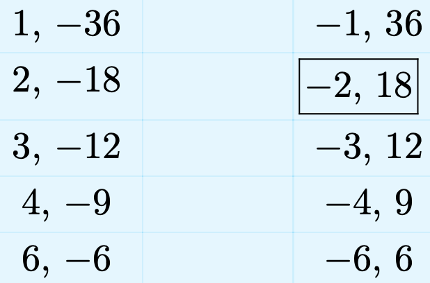
Note that we’ve framed the pair −2, 18. We’ve done this because the sum of this pair of integers equals the coefficient of x in the trinomial expression \(x^2 + 16x − 36\). Use this framed pair to factor the trinomial.

\[x^{2}+16 x-36=(x-2)(x+18) \nonumber \]

It is important that you check your result. Use the distributive property to multiply.

\[\begin{aligned}(x-2)(x+18) &=x(x+18)-2(x+18) \\ &=x^{2}+18 x-2 x-36 \\ &=x^{2}+16 x-36 \end{aligned} \nonumber \]

Thus, our factorization is correct.

Let’s summarize the technique.

Algorithm

To factor the quadratic \(x^2 + bx + c\), proceed as follows:

1. List all the integer pairs whose product equals c.
2. Circle or frame the pair whose sum equals the coefficient of x, namely b. Use this pair to factor the trinomial.

Let’s look at another example.

Example \(\PageIndex{2}\)

Factor the trinomial \(x^{2}-25 x-84\)

Solution

List all the integer pairs whose product is −84.

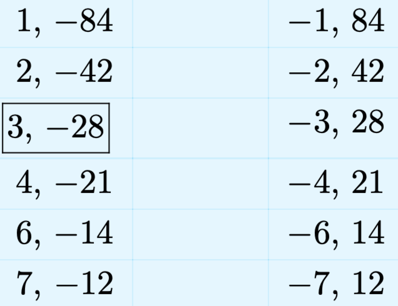
We’ve framed the pair whose sum equals the coefficient of x, namely −25. Use this pair to factor the trinomial.

\[x^{2}-25 x-84=(x+3)(x-28) \nonumber \]

Check

\[\begin{aligned}(x+3)(x-28) &=x(x-28)+3(x-28) \\ &=x^{2}-28 x+3 x-84 \\ &=x^{2}-25 x-84 \end{aligned} \nonumber \]

With experience, there are a number of ideas that will quicken the process.

• As you are listing the integer pairs, should you happen to note that the current pair has the appropriate sum, there is no need to list the remaining integer pairs. Simply halt the process of listing the integer pairs and use the current pair to factor the trinomial.
• Some students are perfectly happy being asked “Can you think of an integer pair whose product is c and whose sum is b (where b and c refer to the coefficients of \(x^2 +bx+c\))?” If you can pick the pair “out of the air” like this, all is well and good.

Use the integer pair to factor the trinomial and don’t bother listing any integer pairs.

Now, let’s investigate how to proceed when the leading coefficient is not 1.

Factoring \(a x^{2}+b x+c\) when \(a \neq 1\)

When \(a \neq 1\), we use a technique called the ac-test to factor the trinomial \(ax^2 + bx + c\). The process is best explained with an example.

Example \(\PageIndex{3}\)

Factor \(2x^2 + 13x − 24\).

Solution

Note that the leading coefficient does not equal 1. Indeed, the coefficient of \(x^2\) in this example is a 2. Therefore, the technique of the previous examples will not work. Thus, we turn to a similar technique called the ac-test.

First, compare \[2 x^{2}+13 x-24 \qquad \text { and } \qquad a x^{2}+b x+c \nonumber \]

and note that a = 2, b = 13, and c = −24. Compute the product of a and c. This is how the technique earns its name “ac-test.”

\[a c=(2)(-24)=-48 \nonumber \]

List all integer pairs whose product is ac = −48.

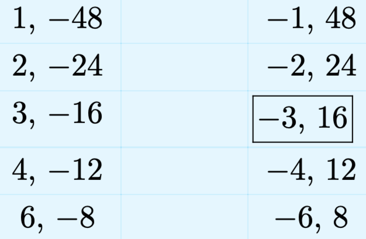
We’ve framed the pair whose sum is b = 13. The next step is to rewrite the trinomial \(2x^2 + 13x − 24\), splitting the middle term into a sum, using our framed integer pair.

\[2 x^{2}+13 x-24=2 x^{2}-3 x+16 x-24 \nonumber \]

We factor an x out of the first two terms, then an 8 out of the last two terms. This process is called factoring by grouping.

\[2 x^{2}-3 x+16 x-24=x(2 x-3)+8(2 x-3) \nonumber \]

We now factor out a common factor of 2x − 3.

\[x(2 x-3)+8(2 x-3)=(x+8)(2 x-3) \nonumber \]

It’s helpful to see the complete process as a coherent unit.

\[\begin{aligned} 2 x^{2}+13 x-24 &=2 x^{2}-3 x+16 x-24 \\ &=x(2 x-3)+8(2 x-3) \\ &=(x+8)(2 x-3) \end{aligned} \nonumber \]

Check

Again, it is important to check the answer by multiplication.

\[\begin{aligned}(x+8)(2 x-3) &=x(2 x-3)+8(2 x-3) \\ &=2 x^{2}-3 x+16 x-24 \\ &=2 x^{2}+13 x-24 \end{aligned} \nonumber \]

Because this is the original trinomial, our solution checks.

Let’s summarize this process.

Algorithm: ac-Test

To factor the quadratic \(ax^2 + bx + c\), proceed as follows:

1. List all integer pairs whose product equals ac.
2. Circle or frame the pair whose sum equals the coefficient of x, namely b.
3. Use the circled pair to express the middle term bx as a sum.
4. Factor by “grouping.”

Let’s look at another example.

Example \(\PageIndex{4}\)

Factor \(3 x^{2}+34 x-24\)

Solution

Compare

\[3 x^{2}+34 x-24 \quad \text { and } \quad a x^{2}+b x+c \nonumber \]

and note that a = 3, b = 34 and c = −24. List all integer pairs whose product equals ac = (3)(−24) = −72.

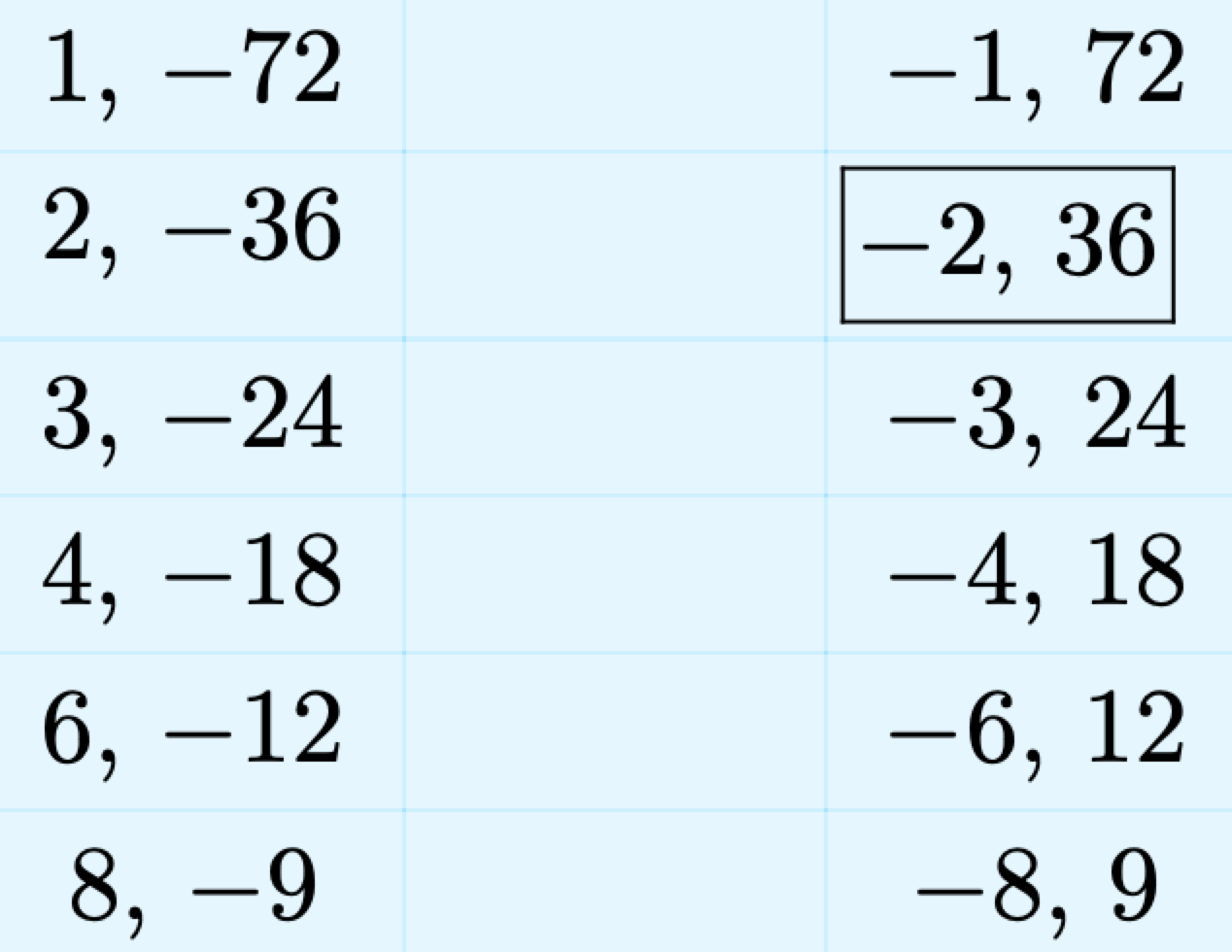
We’ve framed the pair whose sum is the same as b = 34, the coefficient of x in \(3x^2 + 34x − 24\). Again, possible shortcuts are possible. If you can “think” of a pair whose product is ac = −72 and whose sum is b = 34, then it is not necessary to list any integer pairs. Alternatively, if you come across the needed pair as you are listing them, then you can halt the process. There is no need to list the remaining pairs if you have the one you need.

Use the framed pair to express the middle term as a sum, then factor by grouping.

\[\begin{aligned} 3 x^{2}+34 x-24 &=3 x^{2}-2 x+36 x-24 \\ &=x(3 x-2)+12(3 x-2) \\ &=(x+12)(3 x-2) \end{aligned} \nonumber \]

We leave it to the reader to check this result.

Intercepts

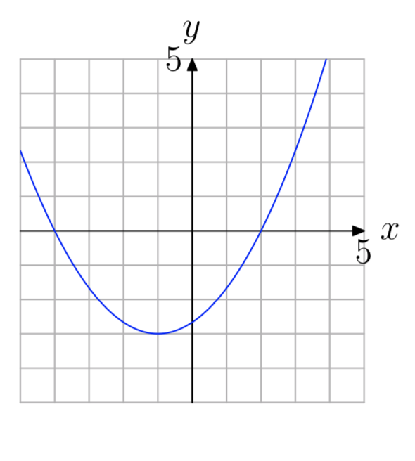
The points where the graph of a function crosses the x-axis are called the x-intercepts of graph of the function. Consider the graph of the quadratic function f in Figure \(\PageIndex{1}\).

Figure \(\PageIndex{1}\): The x- and y-intercepts are key features of any graph.

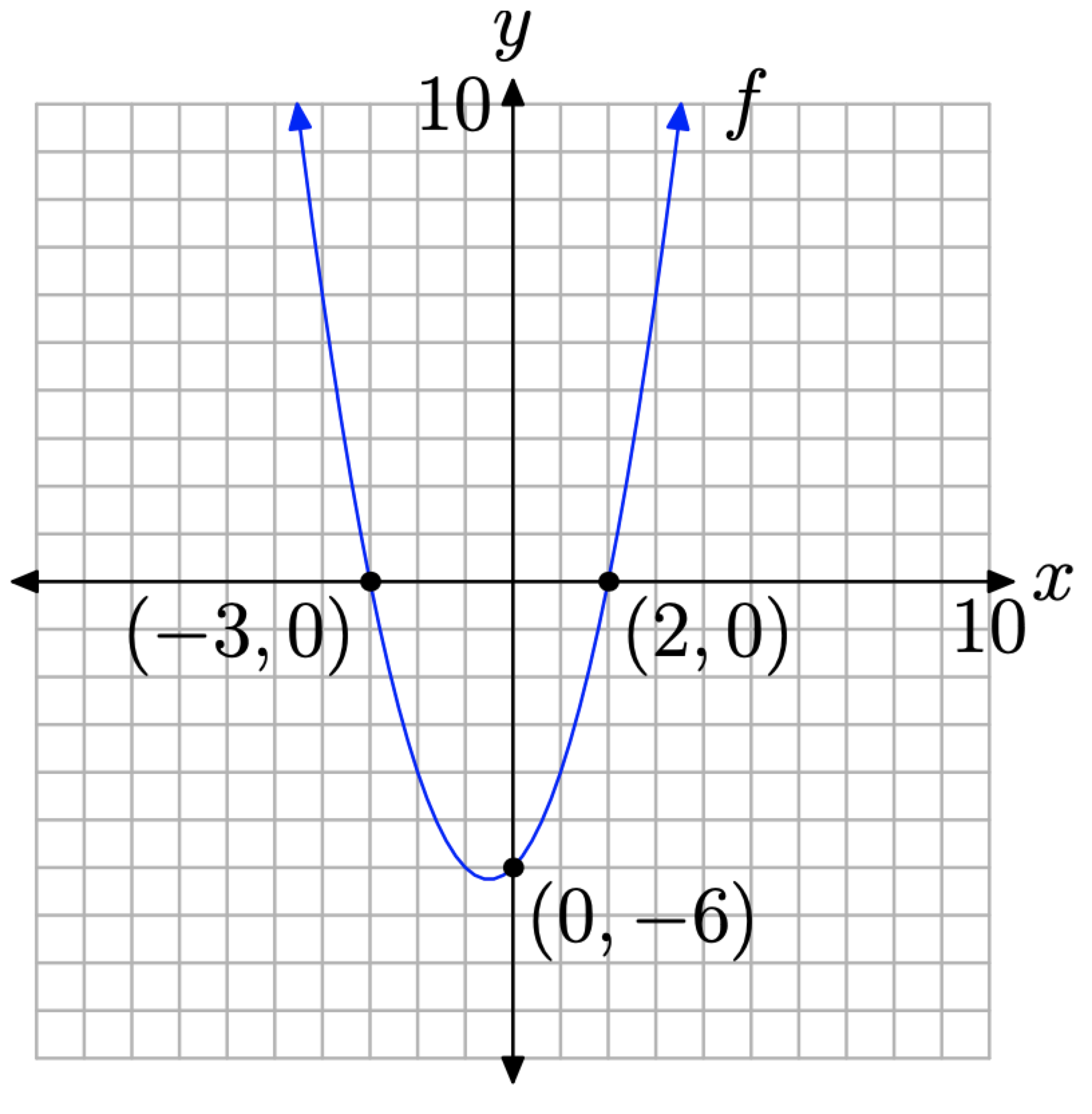
Note that the graph of the f crosses the x-axis at (−3, 0) and (2, 0). These are the x-intercepts of the parabola. Note that the y-coordinate of each x-intercept is zero.

In function notation, the solutions of f(x) = 0 (note the similarity to y = 0) are the x-coordinates of the points where the graph of f crosses the x-axis. Analyzing the graph of f in Figure \(\PageIndex{1}\), we see that both −3 and 2 are solutions of f(x) = 0.

Thus, the process for finding the x-intercepts is clear.

Finding x-intercepts

To find the x-intercepts of the graph of any function, set y = 0 and solve for x. Alternatively, if function notation is used, set f(x) = 0 and solve for x.

Let’s look at an example.

Example \(\PageIndex{5}\)

Find the x-intercepts of the graph of the quadratic function defined by \(y = x^2 + 2x − 48\).

Solution

To find the x-intercepts, first set y = 0.

\[0=x^{2}+2 x-48 \nonumber \]

Next, factor the trinomial on the right. Note that the coefficient of \(x^2\) is 1. We need only think of two integers whose product equals the constant term −48 and whose sum equals the coefficient of x, namely 2. The numbers 8 and −6 come to mind, so the trinomial factors as follows (readers should check this result).

\[0=(x+8)(x-6) \nonumber \]

To complete the solution, we need to use an important property of the real numbers called the zero product property.

Zero Product Property

If a and b are any real numbers such that \[ab = 0 \nonumber \], then either a = 0 or b = 0.

In our case, we have 0 = (x + 8)(x − 6). Therefore, it must be the case that either

\[x+8=0 \qquad \text { or } \qquad x-6=0 \nonumber \]

These equations can be solved independently to produce

\[x=-8 \quad \text { or } \quad x=6 \nonumber \]

Thus, the x-intercepts of the graph of \(y = x^2 + 2x−48\) are located at (−8, 0) and (6, 0).

Let’s look at another example.

Example \(\PageIndex{6}\)

Find the x-intercepts of the graph of the quadratic function \(f(x) = 2x^2 − 7x − 15\).

Solution

To find the x-intercepts of the graph of the quadratic function f, we begin by setting

\[f(x)=0\nonumber \]

Of course, \(f(x) = 2x^2 − 7x − 15\), so we can substitute to obtain

\[2 x^{2}-7 x-15=0 \nonumber \]

We will now use the ac-test to factor the trinomial on the left. Note that ac = (2)(−15) = −30. List the integer pairs whose products equal −30.

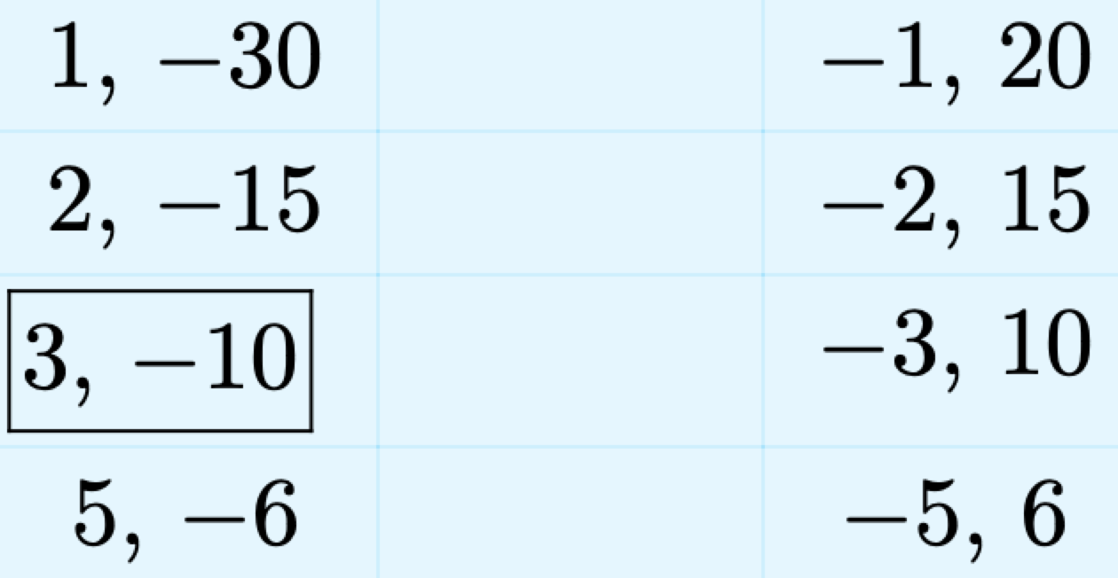
Note that the framed pair sum to the coefficient of x in \(2x^2 − 7x − 15\). Use the framed pair to express the middle term as a sum, then factor by grouping

\[\begin{aligned} 2 x^{2}-7 x-15 &=0 \\ 2 x^{2}+3 x-10 x-15 &=0 \\ x(2 x+3)-5(2 x+3) &=0 \\(x-5)(2 x+3) &=0 \end{aligned} \nonumber \]

Now we can use the zero product property. Either

\[x-5=0 \qquad \text { or } \qquad 2 x+3=0 \nonumber \]

Each of these can be solved independently to obtain

\[x=5 \qquad \text { or } \qquad x=-3 / 2 \nonumber \]

Thus, the x-intercepts of the graph of the quadratic function \(f(x) = 2x^2 − 7x − 15\) are located at (−3/2, 0) and (5, 0).

One more definition is in order.

Definition 7: Zeros of a Function

he solutions of f(x) = 0 are called the zeros of the function f.

Thus, in the last example, both −3/2 and 5 are zeros of the quadratic function \(f(x) = 2x^2−7x−15\). Note the intimate relationship between the zeros of the quadratic function and the x-intercepts of the graph. Note that −3/2 is a zero and (−3/2, 0) is an x-intercept. Similarly, 5 is a zero and (5, 0) is an x-intercept.

The graphing calculator can be used to find the zeros of a function.

Example \(\PageIndex{7}\)

Use the graphing calculator to find the zeros of the function \(f(x) = 2x^2 − 7x − 15\).

Solution

Enter the function \(f(x) = 2x^2 − 7x − 15\) into Y1 in the Y= menu; then adjust the window parameters as shown in Figure \(\PageIndex{2}\)(b). Push the GRAPH button to produce the parabola shown in Figure \(\PageIndex{2}\)(c).

To find a zero of the function, proceed as follows:

Figure \(\PageIndex{2}\). Plotting the quadratic function \(f(x) = 2x^2 − 7x − 15\).

• Press 2nd TRACE to open the CALCULATE window shown in Figure \(\PageIndex{3}\)(a). From this menu, select 2:zero.
• The calculator responds by asking for a “Left bound.” Use the arrow keys to move the cursor slightly to the left of the leftmost x-intercept, as shown in Figure \(\PageIndex{3}\)(b). Press the ENTER key.
• The calculator responds by asking for a “Right bound.” Use the arrow keys to move the cursor slightly to the right of the leftmost x-intercept, as shown in Figure \(\PageIndex{3}\)(c). Press the ENTER key.
• The calculator responds by asking for a “Guess.” You may use the arrow keys to select a starting x-value any where between the left- and right-bounds you selected (note that the calculator marks these on the screen in Figure \(\PageIndex{3}\)(d)). However, the cursor already lies between these marks, so we typically just hit ENTER at this point. We suggest you do so also.

Figure \(\PageIndex{3}\). Using the zero utility to find an x-intercept.

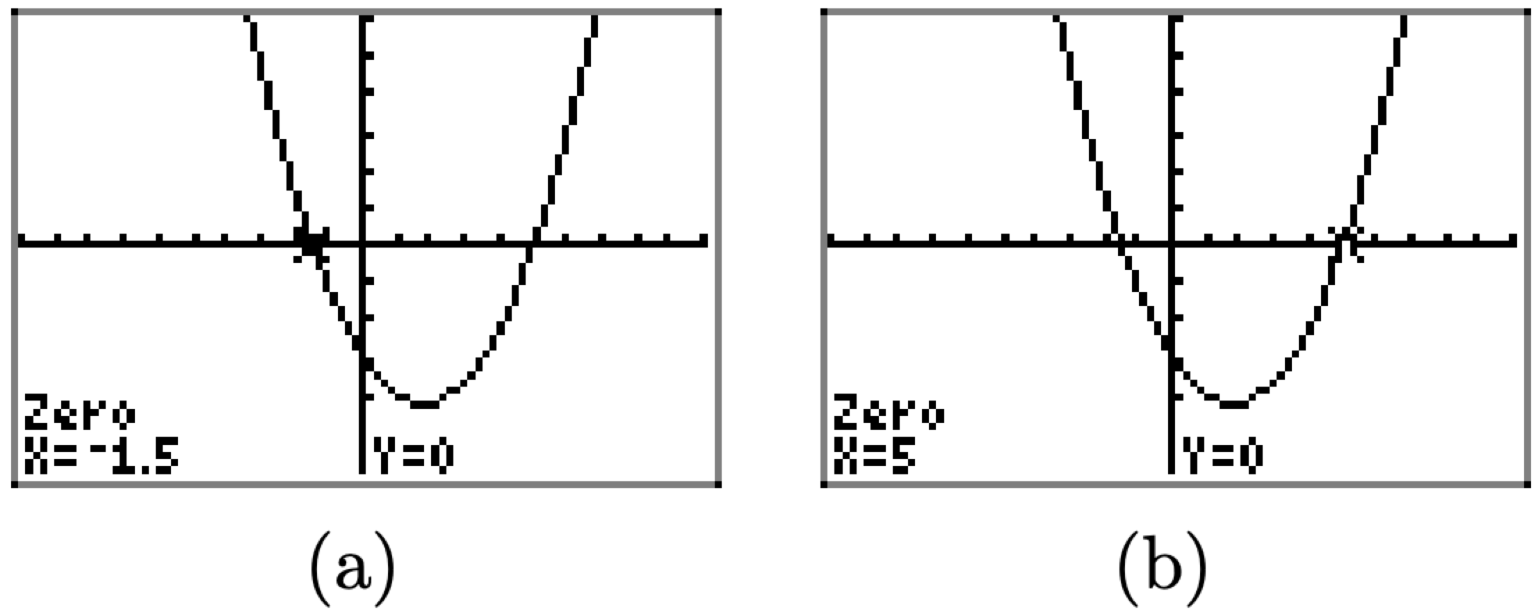
The calculator responds by marking the x-intercept and reporting its x-value at the bottom of the screen, as shown in Figure \(\PageIndex{4}\)(a). This is one of the zeros of the function. Note that this value of −1.5 agrees nicely with our hand calculated result −3/2 in Example \(\PageIndex{6}\). We followed precisely the same procedure outlined above to find the second x-intercept shown in Figure \(\PageIndex{4}\)(b). Note that it also agrees with the hand calculated solution of Example \(\PageIndex{6}\).

In a similar vein, the point where the graph of a function crosses the y-axis is called the y-intercept of the graph of the function. In Figure \(\PageIndex{1}\) the y-intercept of the parabola is (0, −6). Note that the x-coordinate of this y-intercept is zero.

Thus, the process for finding y-intercepts should be clear.

Figure \(\PageIndex{4}\): The zeros of \(f(x) − 2x^2 − 7x − 15\).

Finding Y-Intercepts

To find the y-intercepts of the graph of any function, set \(x = 0\) and solve for \(y\). Alternatively, if function notation is used, simply evaluate f(0).

Example \(\PageIndex{8}\)

Find the y-intercept of the quadratic function defined by \(f(x) = x^2 − 3x − 11\).

Solution

Evaluate the function at x = 0.

\[f(0)=(0)^{2}-3(0)-11=-11 \nonumber \]

The coordinates of the y-intercept are (0, −11).

Putting it All Together

We will find both x- and y-intercepts extremely useful when drawing the graph of a quadratic function.

Example \(\PageIndex{9}\)

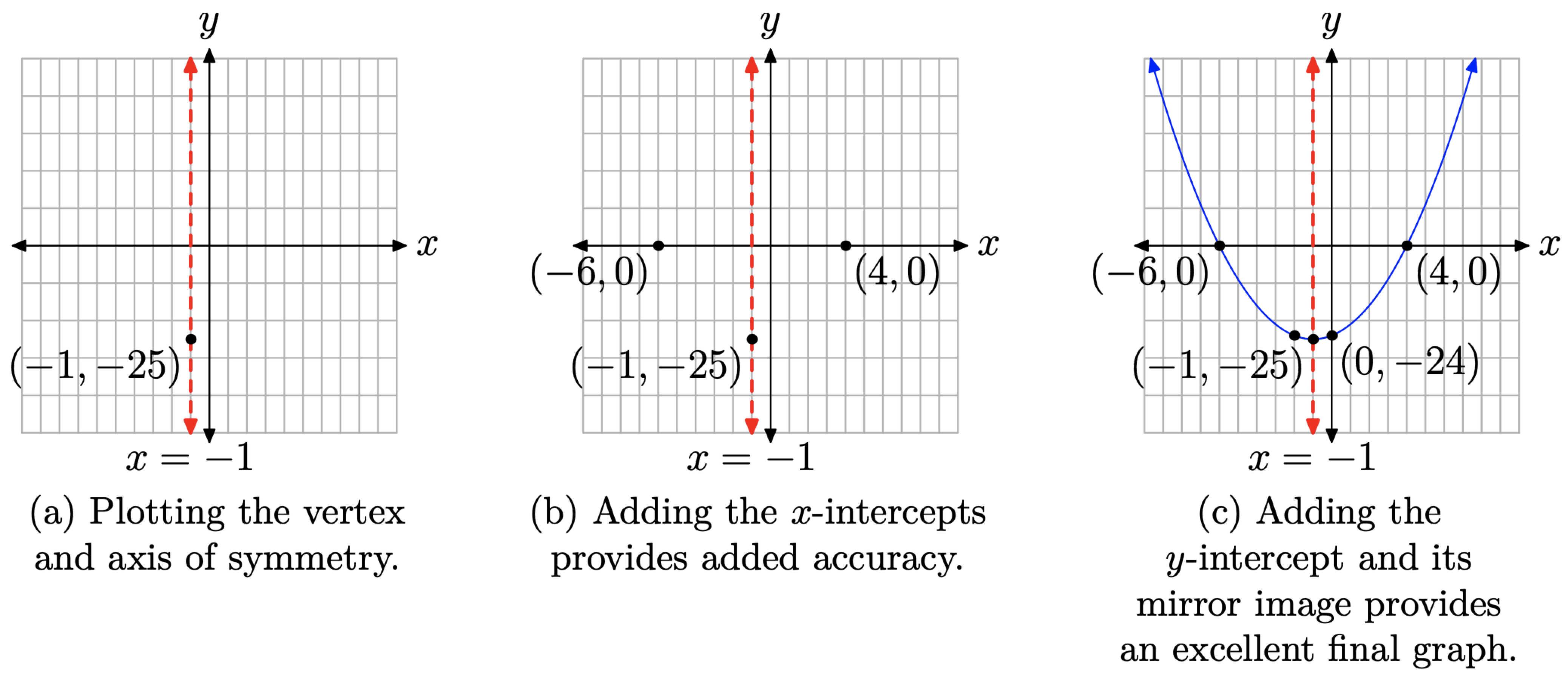
Place the quadratic function \(y = x^2 + 2x − 24\) in vertex form. Plot the vertex and axis of symmetry and label them with their coordinates and equation, respectively. Find and plot the x- and y-intercepts of the parabola and label them with their coordinates.

Solution

Take half of the coefficient of x, square, then add and subtract this amount to balance the equation. Factor and combine coefficients.

\[\begin{array}{l}{y=x^{2}+2 x+1-1-24} \\ {y=(x+1)^{2}-25}\end{array} \nonumber \]

The graph is a parabola that opens upward; it is shifted 1 unit to the left and 25 units downward. This information is enough to plot and label the vertex, then plot and label the axis of symmetry, as shown in Figure \(\PageIndex{5}\)(a).

To find the x-intercepts, let y = 0 in \(y = x^2 + 2x − 24\).

\[0=x^{2}+2 x-24 \nonumber \]

The leading coefficient is a 1. The integer pair −4 and 6 has product −24 and sum 2. Thus, the right-hand side factors as follows.

\[0=(x+6)(x-4) \nonumber \]

In order that this product equals zero, either

\[x+6=0 \qquad \text { or } \qquad x-4=0 \nonumber \]

Solve each of these linear equations independently.

\[x=-6 \qquad \text { or } \qquad x=4 \nonumber \]

Recall that we let y = 0. We’ve found two solutions, x = −6 and x = 4. Thus, we have x-intercepts at (−6, 0) and (4, 0), as pictured in Figure \(\PageIndex{5}\)(b).

Finally, to find the y-intercept, let x = 0 in \(y = x^2+2x−24\). With this substitution, y = −24. Thus, the y-intercept is (0, −24), as pictured in Figure \(\PageIndex{5}\)(c). Note that we’ve also included the mirror image of the y-intercept across the axis of symmetry.

Figure \(\PageIndex{5}\)

Let’s look at one final example.

Example \(\PageIndex{10}\)

Plot the parabola represented by the equation \(f(x) = −2x^2−7x+15\). Plot and label the vertex, axis of symmetry, and the x- and y-intercepts.

Solution

First, factor out a −2.

\[f(x)=-2\left[x^{2}+\frac{7}{2} x-\frac{15}{2}\right] \nonumber \]

Half of 7/2 is 7/4. Squared, this amounts to 49/16. Add and subtract this last amount to keep the equation balanced.

\[f(x)=-2\left[x^{2}+\frac{7}{2} x+\frac{49}{16}-\frac{49}{16}-\frac{15}{2}\right] \nonumber \]

The first three terms inside the parentheses form a perfect square trinomial. The last two constants are combined with a common denominator.

\[\begin{array}{l}{f(x)=-2\left[\left(x^{2}+\frac{7}{2} x+\frac{49}{16}\right)-\frac{49}{16}-\frac{120}{16}\right]} \\ {f(x)=-2\left[\left(x+\frac{7}{4}\right)^{2}-\frac{169}{16}\right]}\end{array} \nonumber \]

Finally, redistribute the −2.

\[f(x)=-2\left(x+\frac{7}{4}\right)^{2}+\frac{169}{8} \nonumber \]

The graph of this last equation is a parabola that opens downward, translated 7/4 units to the left and 169/8 units upward. This is enough information to plot and label the vertex and axis of symmetry, as shown in Figure \(\PageIndex{6}\)(a).

To find the y-intercepts, set f(x) = 0 in \(f(x) = −2x^2 − 7x + 15\). We will also multiply both sides of the resulting equation by −1.

\[\begin{array}{l}{0=-2 x^{2}-7 x+15} \\ {0=2 x^{2}+7 x-15}\end{array} \nonumber \]

After comparing \(2x^2 + 7x − 15\) with \(ax^2 + bx + c\), we note that the integer pair −3 and 10 have product equal to ac = −30 and sum equal to b = 7. Use this pair to express the middle term of \(2x^2 + 7x − 15\) as a sum and then factor by grouping.

\[\begin{array}{l}{0=2 x^{2}-3 x+10 x-15} \\ {0=x(2 x-3)+5(2 x-3)} \\ {0=(x+5)(2 x-3)}\end{array} \nonumber \]

By the zero product property, either \[x+5=0 \qquad \text { or } \qquad 2 x-3=0 \nonumber \]

Solve these linear equations independently. \[x=-5 \qquad \text { or } \qquad x=\frac{3}{2} \nonumber \]

These x-values are the zeros of f (they make f(x) = 0), so we have x-intercepts at (−5, 0) and (3/2, 0), as shown in Figure \(\PageIndex{6}\)(b).

Figure \(\PageIndex{6}\)

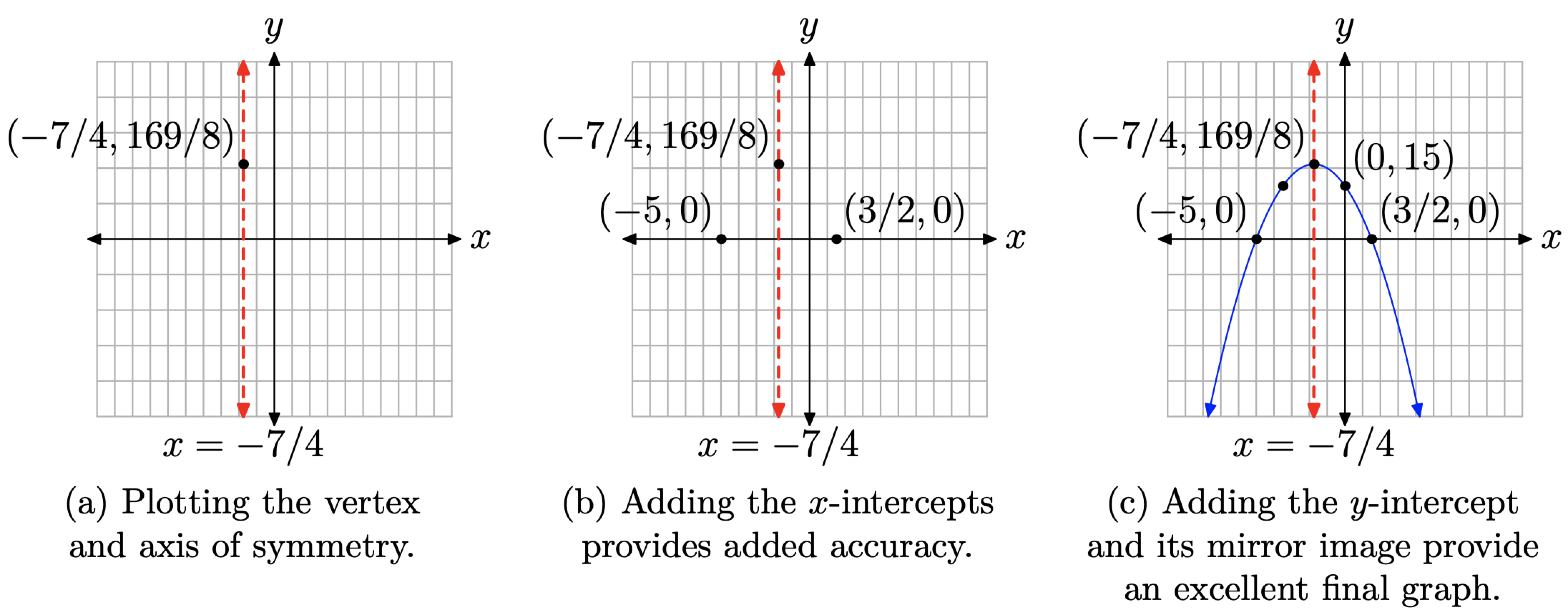
Finally, to find the y-intercept, set x = 0 in \(f(x) = −2x^2 − 7x + 15\) to get f(0) = 15. Note the positioning of the y-intercept (0, 15) and its mirror image across the axis of symmetry in Figure \(\PageIndex{6}\)(c).

Exercise

In Exercises 1-8, factor the given quadratic polynomial.

Exercise \(\PageIndex{1}\)

\(x^2+9x+14\)

Answer

(x+2)(x+7)

Exercise \(\PageIndex{2}\)

\(x^2+6x+5\)

Exercise \(\PageIndex{3}\)

\(x^2+10x+9\)

Answer

(x+9)(x+1)

Exercise \(\PageIndex{4}\)

\(x^2+4x−21\)

Exercise \(\PageIndex{5}\)

\(x^2−4x−5\)

Answer

(x−5)(x+1)

Exercise \(\PageIndex{6}\)

\(x^2+7x−8\)

Exercise \(\PageIndex{7}\)

\(x^2−7x+12\)

Answer

(x−4)(x−3)

Exercise \(\PageIndex{8}\)

\(x^2+5x−24\)

In Exercises 9-16, find the zeros of the given quadratic function.

Exercise \(\PageIndex{9}\)

\(f(x) = x^2−2x−15\)

Answer

Zeros: x = −3, x = 5

Exercise \(\PageIndex{10}\)

\(f(x) = x^2+4x−32\)

Exercise \(\PageIndex{11}\)

\(f(x) = x^2+10x−39\)

Answer

Zeros: x = −13, x = 3

Exercise \(\PageIndex{12}\)

\(f(x) = x^2+4x−45\)

Exercise \(\PageIndex{13}\)

\(f(x) = x^2−14x+40\)

Answer

Zeros: x = 4, x = 10

Exercise \(\PageIndex{14}\)

\(f(x) = x^2−5x−14\)

Exercise \(\PageIndex{15}\)

\(f(x) = x^2+9x−36\)

Answer

Zeros: x = −12, x = 3

Exercise \(\PageIndex{16}\)

\(f(x) = x^2+11x−26\)

In Exercises 17-22, perform each of the following tasks for the quadratic functions.

1. Load the function into Y1 of the Y= of your graphing calculator. Adjust the window parameters so that the vertex is visible in the viewing window.
2. Set up a coordinate system on your homework paper. Label and scale each axis with xmin, xmax, ymin, and ymax. Make a reasonable copy of the image in the viewing window of your calculator on this coordinate system and label it with its equation.
3. Use the zero utility on your graphing calculator to find the zeros of the function. Use these results to plot the x-intercepts on your coordinate system and label them with their coordinates.
4. Use a strictly algebraic technique (no calculator) to find the zeros of the given quadratic function. Show your work next to your coordinate system. Be stubborn! Work the problem until your algebraic and graphically zeros are a reasonable match.

Exercise \(\PageIndex{17}\)

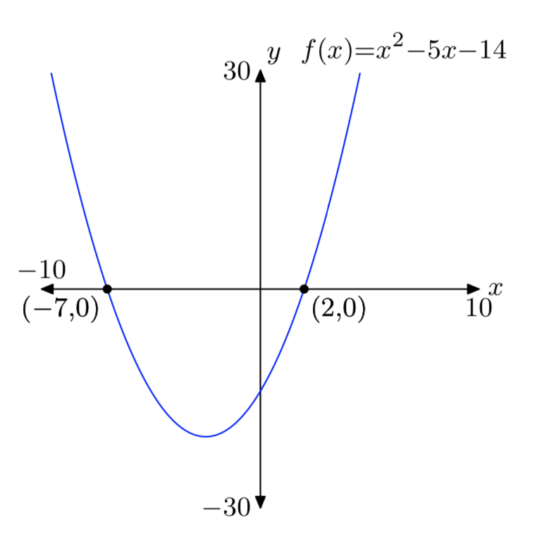
\(f(x) = x^2+5x−14\)

Answer

Exercise \(\PageIndex{18}\)

\(f(x) = x^2+x−20\)

Exercise \(\PageIndex{19}\)

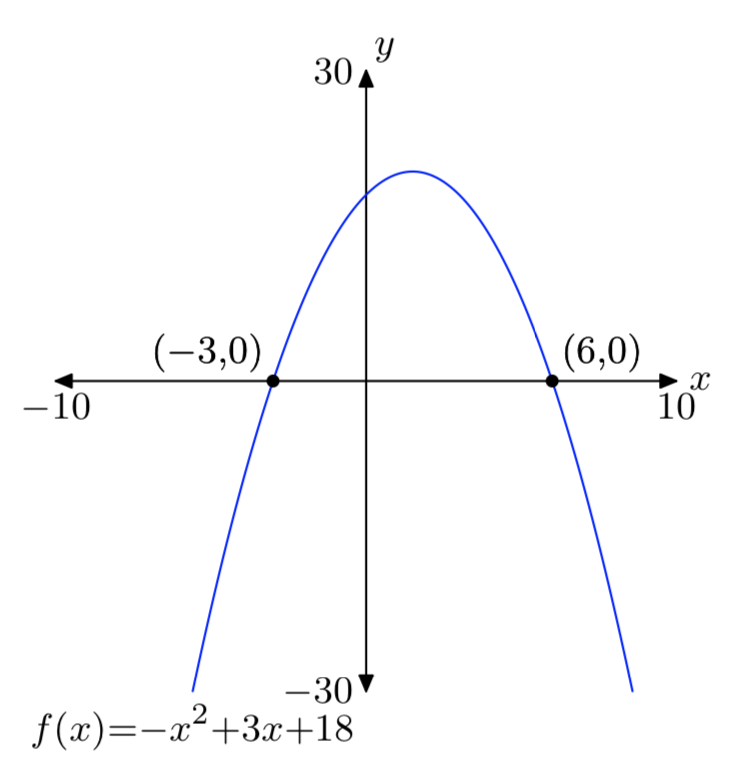
\(f(x) = −x^2+3x+18\)

Answer

Exercise \(\PageIndex{20}\)

\(f(x) = −x^2+3x+40\)

Exercise \(\PageIndex{21}\)

\(f(x) = x^2−16x−36\)

Answer

Exercise \(\PageIndex{22}\)

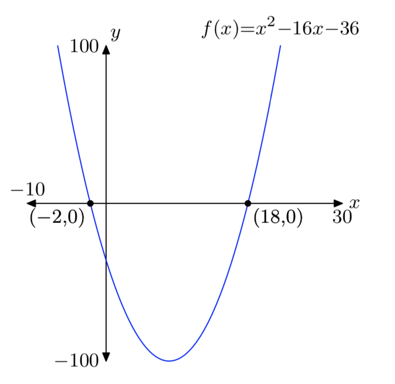
\(f(x) = x^2+4x−96\)

In Exercises 23-30, perform each of the following tasks for the given quadratic function.

1. Set up a coordinate system on graph paper. Label and scale each axis. Remember to draw all lines with a ruler.
2. Use the technique of completing the square to place the quadratic function in vertex form. Plot the vertex on your coordinate system and label it with its coordinates. Draw the axis of symmetry on your coordinate system and label it with its equation.
3. Use a strictly algebraic technique (no calculators) to find the x-intercepts of the graph of the given quadratic function. Plot them on your coordinate system and label them with their coordinates.
4. Find the y-intercept of the graph of the quadratic function. Plot the y-intercept on your coordinate system and its mirror image across the axis of symmetry, then label these points with their coordinates.
5. Using all the information plotted, draw the graph of the quadratic function and label it with the vertex form of its equation. Use interval notation to describe the domain and range of the quadratic function.

Exercise \(\PageIndex{23}\)

\(f(x) = x^2+2x−8\)

Answer

Domain = (\(−\infty, \infty\)), Range = [−9, \(\infty\))

Exercise \(\PageIndex{24}\)

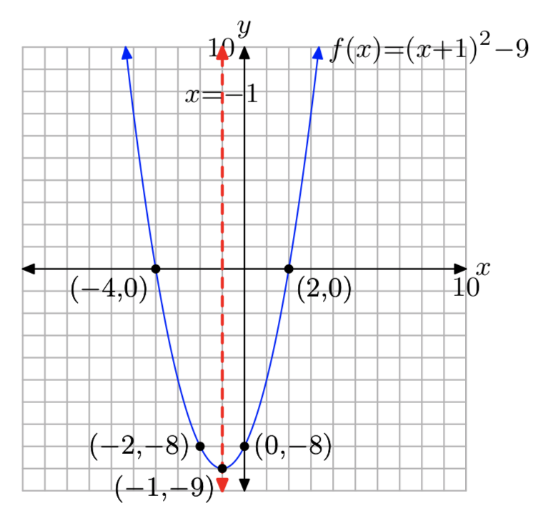
\(f(x) = x^2−6x+8\)

Exercise \(\PageIndex{25}\)

\(f(x) = x^2+4x−12\)

Answer

Domain = (\(−\infty, \infty\)), Range = [−16, \(\infty\))

Exercise \(\PageIndex{26}\)

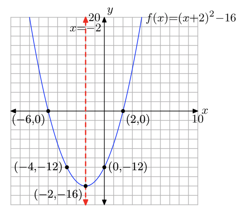
\(f(x) = x^2+8x+12\)

Exercise \(\PageIndex{27}\)

\(f(x) = −x^2−2x+8\)

Answer

Domain = (\(−\infty, \infty\)), Range = (\(−\infty\), 9]

Exercise \(\PageIndex{28}\)

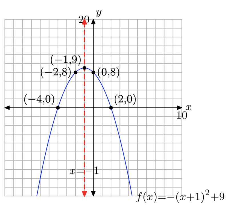
\(f(x) = −x^2−2x+24\)

Exercise \(\PageIndex{29}\)

\(f(x) = −x^2−8x+48\)

Answer

Domain = (\(−\infty, \infty\)), Range = (\(−\infty\), 64]

Exercise \(\PageIndex{30}\)

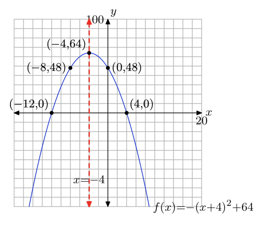
\(f(x) = −x^2−8x+20\)

In Exercises 31-38, factor the given quadratic polynomial.

Exercise \(\PageIndex{31}\)

\(42x^2+5x−2\)

Answer

(7x+2)(6x−1)

Exercise \(\PageIndex{32}\)

\(3x^2+7x−20\)

Exercise \(\PageIndex{33}\)

\(5x^2−19x+12\)

Answer

(x−3)(5x−4)

Exercise \(\PageIndex{34}\)

\(54x^2−3x−1\)

Exercise \(\PageIndex{35}\)

\(−4x^2+9x−5\)

Answer

(4x−5)(−x+1)

Exercise \(\PageIndex{36}\)

\(3x^2−5x−12\)

Exercise \(\PageIndex{37}\)

\(2x^2−3x−35\)

Answer

(2x+7)(x−5)

Exercise \(\PageIndex{38}\)

\(−6x^2+25x+9\)

In Exercises 39-46, find the zeros of the given quadratic functions.

Exercise \(\PageIndex{39}\)

\(f(x) = 2x^2−3x−20\)

Answer

Zeros: \(x = −\frac{5}{2}\), x = 4

Exercise \(\PageIndex{40}\)

\(f(x) = 2x^2−7x−30\)

Exercise \(\PageIndex{41}\)

\(f(x) = −2x^2+x+28\)

Answer

Zeros: \(x = −\frac{7}{2}\), x = 4

Exercise \(\PageIndex{42}\)

\(f(x) = −2x^2+15x−22\)

Exercise \(\PageIndex{43}\)

\(f(x) = 3x^2−20x+12\)

Answer

Zeros: \(x = \frac{2}{3}\), x = 6

Exercise \(\PageIndex{44}\)

\(f(x) = 4x^2+11x−20\)

Exercise \(\PageIndex{45}\)

\(f(x) = −4x^2+4x+15\)

Answer

Zeros: \(x = −\frac{3}{2}\), \(x = \frac{5}{2}\)

Exercise \(\PageIndex{46}\)

\(f(x) = −6x^2−x+12\)

In Exercises 47-52, perform each of the following tasks for the given quadratic functions.

1. Load the function into Y1 of the Y= of your graphing calculator. Adjust the window parameters so that the vertex is visible in the viewing window.
2. Set up a coordinate system on your homework paper. Label and scale each axis with xmin, xmax, ymin, and ymax. Make a reasonable copy of the image in the viewing window of your calculator on this coordinate system and label it with its equation.
3. Use the zero utility on your graphing calculator to find the zeros of the function. Use these results to plot the x-intercepts on your coordinate system and label them with their co- ordinates.
4. Use a strictly algebraic technique (no calculator) to find the zeros of the given quadratic function. Show your work next to your coordinate system. Be stubborn! Work the problem until your algebraic and graphically zeros are a reasonable match.

Exercise \(\PageIndex{47}\)

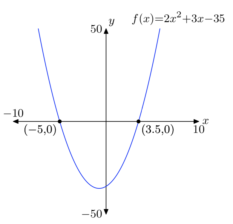
\(f(x) = 2x^2+3x−35\)

Answer

Exercise \(\PageIndex{48}\)

\(f(x) = 2x^2−5x−42\)

Exercise \(\PageIndex{49}\)

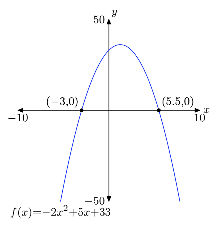
\(f(x) = −2x^2+5x+33\)

Answer

Exercise \(\PageIndex{50}\)

\(f(x) = −2x^2−5x+52\)

Exercise \(\PageIndex{51}\)

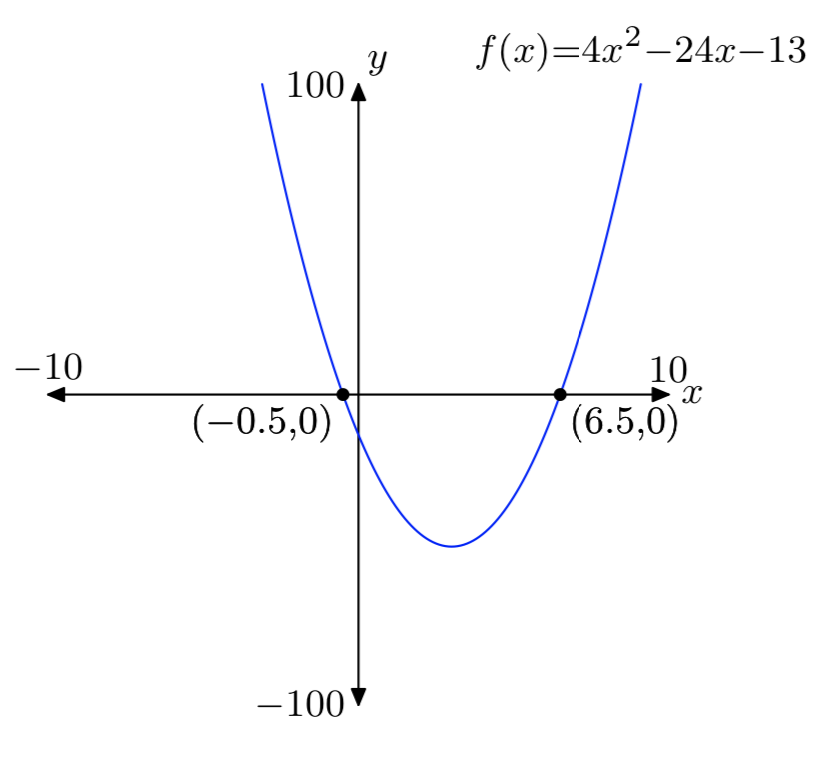
\(f(x) = 4x^2−24x−13\)

Answer

Exercise \(\PageIndex{52}\)

\(f(x) = 4x^2+24x−45\)

In Exercises 53-60, perform each of the following tasks for the given quadratic functions.

1. Set up a coordinate system on graph paper. Label and scale each axis. Remember to draw all lines with a ruler.
2. Use the technique of completing the square to place the quadratic function in vertex form. Plot the vertex on your coordinate system and label it with its coordinates. Draw the axis of symmetry on your coordinate system and label it with its equation.
3. Use a strictly algebraic method (no calculators) to find the x-intercepts of the graph of the quadratic function. Plot them on your coordinate system and label them with their coordinates.
4. Find the y-intercept of the graph of the quadratic function. Plot the y-intercept on your coordinate system and its mirror image across the axis of symmetry, then label these points with their coordinates.
5. Using all the information plotted, draw the graph of the quadratic function and label it with the vertex form of its equation. Use interval notation to describe the domain and range of the quadratic function.

Exercise \(\PageIndex{53}\)

\(f(x) = 2x^2−8x−24\)

Answer

Domain = (\(−\infty, \infty\)), Range = [−32, \(\infty\))

Exercise \(\PageIndex{54}\)

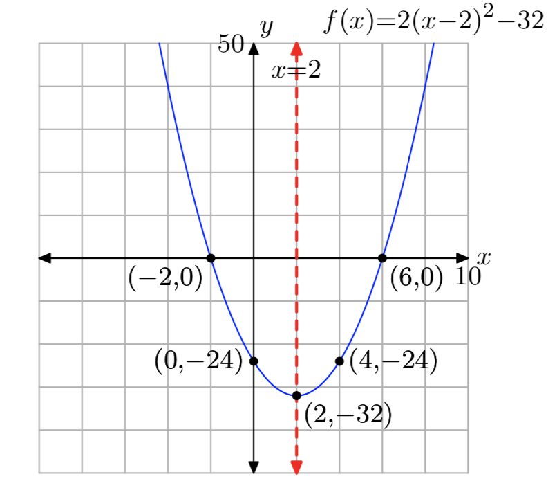
\(f(x) = 2x^2−4x−6\)

Exercise \(\PageIndex{55}\)

\(f(x) = −2x^2−4x+16\)

Answer

Domain = (\(−\infty, \infty\)), Range = (\(−\infty\), 18]

Exercise \(\PageIndex{56}\)

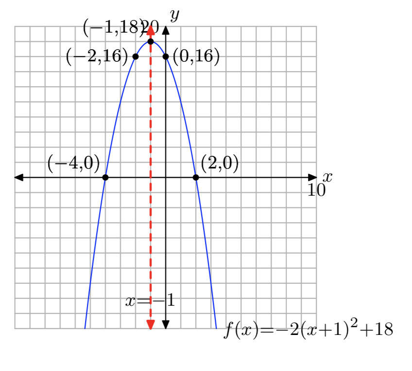
\(f(x) = −2x^2−16x+40\)

Exercise \(\PageIndex{57}\)

\(f(x) = 3x^2+18x−48\)

Answer

Domain = (\(−\infty, \infty\)), Range = [−75, \(\infty\))

Exercise \(\PageIndex{58}\)

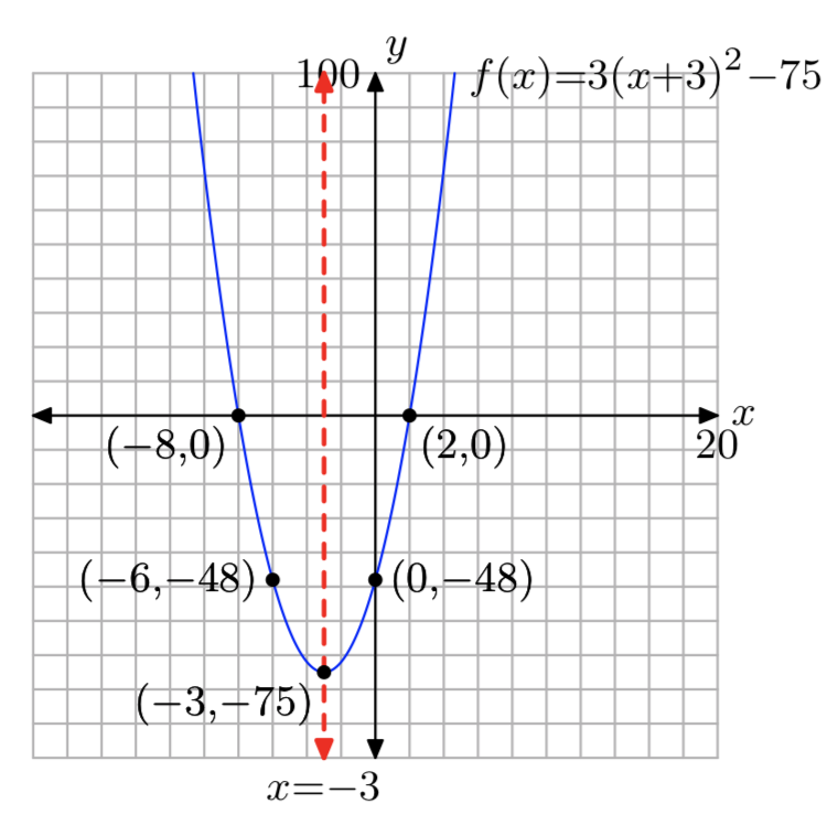
\(f(x) = 3x^2+18x−216\)

Exercise \(\PageIndex{59}\)

\(f(x) = 2x^2+10x−48\)

Answer

Domain = (\(−\infty, \infty\)), Range = [−\(\frac{121}{2}\), \(\infty\))

Exercise \(\PageIndex{60}\)

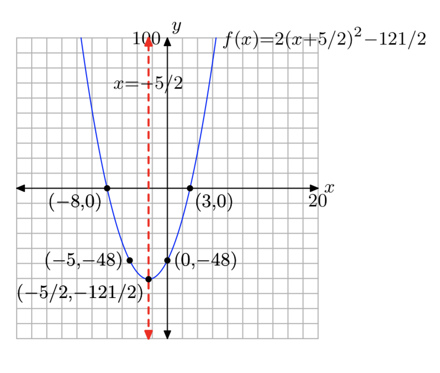
\(f(x) = 2x^2−10x−100\)

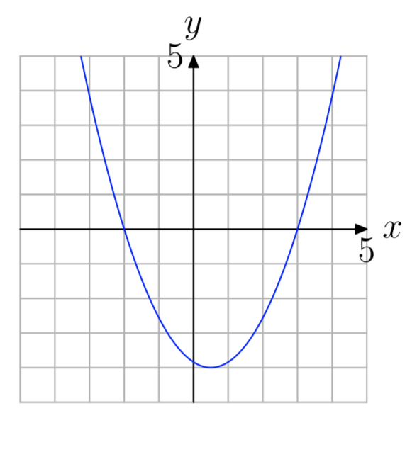
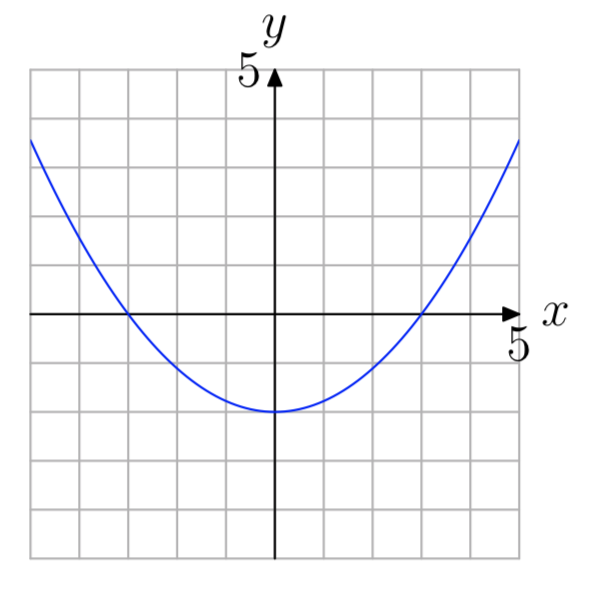
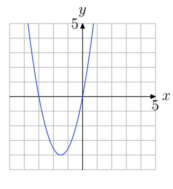
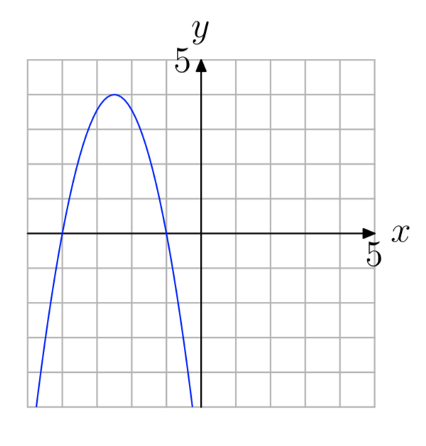
In Exercises 61-66, Use the graph of \(f(x) = ax^2+bx+c\) shown to find all solutions of the equation f(x) = 0. (Note: Every solution is an integer.)

Exercise \(\PageIndex{61}\)

Answer

−2, 3

Exercise \(\PageIndex{62}\)

Exercise \(\PageIndex{63}\)

Answer

−3, 0

Exercise \(\PageIndex{64}\)

Exercise \(\PageIndex{65}\)

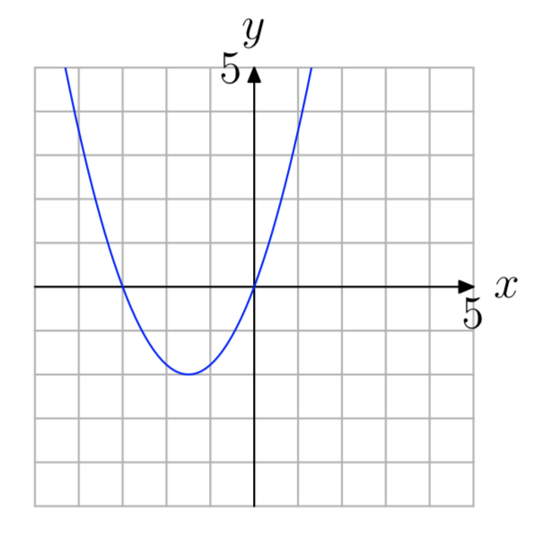
Answer

−3, 0

Exercise \(\PageIndex{66}\)