11.9: Parametric Equations

The Etch A Sketch was a toy invented in the late 1950s by French electrician André Cassagnes. The toy has a thick, flat gray screen in a red plastic frame with two white knobs on the front of the frame in the lower corners, as seen in Figure 1. Twisting the knobs moves a stylus that displaces aluminum powder on the back of the screen, leaving a solid line.

Figure 1: The Etch A Sketch

The left knob controls the horizontal movement of the stylus, while the right knob controls the vertical movement. In a very real way, these knobs represent functions of their respective rotational positions. That is, if you rotate the left knob counterclockwise by $90^{ \circ }$, the stylus will have moved to the left, say, 1 centimeter. Therefore, if $\alpha$ is the angle through which we have rotated the left knob, there is a single horizontal position of the stylus related to $\alpha$. Likewise, if $\beta$ is the angle through which we have rotated the right knob, there is a single vertical position of the stylus related to $\beta$.

Despite the knobs being functions of the horizontal and vertical positions, the artwork generated by an Etch A Sketch does not need to be a function of a horizontal or a vertical variable - it does not need to pass the Vertical nor the Horizontal Line Tests (as Figure 1 showcases). In this chapter, we investigate how to represent simple forms of "Etch A Sketch" curves mathematically.

As we have seen in Exercises 53 - 56 in Section 1.2, Chapter 7 and most recently in Section 11.5, there are scores of interesting curves which, when plotted in the $xy$-plane, neither represent $y$ as a function of $x$ nor $x$ as a function of $y$. In this section, we present a new concept which allows us to use functions to study these kinds of curves. To motivate the idea, we imagine a bug crawling across a table top starting at the point $O$ and tracing out a curve $C$ in the plane, as shown below.

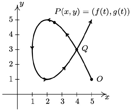
The curve $C$ does not represent $y$ as a function of $x$ because it fails the Vertical Line Test and it does not represent $x$ as a function of $y$ because it fails the Horizontal Line Test. However, since the bug can be in only one place $P(x, y)$ at any given time $t$, we can define the $x$-coordinate of $P$ as a function of $t$ and the $y$-coordinate of $P$ as a (usually, but not necessarily) different function of $t$. (Traditionally, $f(t)$ is used for $x$ and $g(t)$ is used for $y$.) The independent variable $t$ in this case is called a parameter and the system of equations $$\left\{\begin{array}{l} x=f(t) \\ y=g(t) \end{array}\right.\nonumber$$ is called a system of parametric equations or a parametrization of the curve $C$.¹ The parametrization of $C$ endows it with an orientation and the arrows on $C$ indicate motion in the direction of increasing values of $t$. In this case, our bug starts at the point $O$, travels upwards to the left, then loops back around to cross its path² at the point $Q$ and finally heads off into the first quadrant. It is important to note that the curve itself is a set of points and as such is devoid of any orientation. The parametrization determines the orientation and as we shall see, different parametrizations can determine different orientations. If all of this seems hauntingly familiar, it should. By definition, the system of equations $\{x=\cos (t), y=\sin (t)$ parametrizes the Unit Circle, giving it a counter-clockwise orientation. More generally, the equations of circular motion $\{x=r \cos (\omega t), y=r \sin (\omega t)$ developed on page 732 in Section 10.2.1 are parametric equations which trace out a circle of radius $r$ centered at the origin. If $\omega>0$, the orientation is counterclockwise; if $\omega<0$, the orientation is clockwise. The angular frequency $\omega$ determines ‘how fast’ the object moves around the circle. In particular, the equations $\left\{x=2960 \cos \left(\frac{\pi}{12} t\right), y=2960 \sin \left(\frac{\pi}{12} t\right)\right.$ that model the motion of Lakeland Community College as the earth rotates (see Example 10.2.7 in Section 10.2) parameterize a circle of radius 2960 with a counter-clockwise rotation which completes one revolution as $t$ runs through the interval [0, 24). It is time for another example

Example 11.10.1

Sketch the curve described by $\left\{\begin{array}{l} x=t^{2}-3 \\ y=2 t-1 \end{array} \text { for } t \geq-2\right..$

Solution

We follow the same procedure here as we have time and time again when asked to graph anything new – choose friendly values of $t$, plot the corresponding points and connect the results in a pleasing fashion. Since we are told $t \geq-2$, we start there and as we plot successive points, we draw an arrow to indicate the direction of the path for increasing values of $t$.

The curve sketched out in Example 11.10.1 certainly looks like a parabola, and the presence of the $t^{2}$ term in the equation $x=t^{2}-3$ reinforces this hunch. Since the parametric equations $\left\{x=t^{2}-3, y=2 t-1\right.$ given to describe this curve are a system of equations, we can use the technique of substitution as described in Section 8.7 to eliminate the parameter $t$ and get an equation involving just $x$ and $y$. To do so, we choose to solve the equation $y=2 t-1$ for $t$ to get $t=\frac{y+1}{2}$. Substituting this into the equation $x=t^{2}-3$ yields $x=\left(\frac{y+1}{2}\right)^{2}-3$ or, after some rearrangement, $(y+1)^{2}=4(x+3)$. Thinking back to Section 7.3, we see that the graph of this equation is a parabola with vertex $(−3, −1)$ which opens to the right, as required. Technically speaking, the equation $(y+1)^{2}=4(x+3)$ describes the entire parabola, while the parametric equations $\left\{x=t^{2}-3, y=2 t-1 \text { for } t \geq-2\right.$ describe only a portion of the parabola. In this case,³ we can remedy this situation by restricting the bounds on $y$. Since the portion of the parabola we want is exactly the part where $y \geq-5$, the equation $(y+1)^{2}=4(x+3)$ coupled with the restriction $y \geq-5$ describes the same curve as the given parametric equations. The one piece of information we can never recover after eliminating the parameter is the orientation of the curve.

Eliminating the parameter and obtaining an equation in terms of $x$ and $y$, whenever possible, can be a great help in graphing curves determined by parametric equations. If the system of parametric equations contains algebraic functions, as was the case in Example 11.10.1, then the usual techniques of substitution and elimination as learned in Section 8.7 can be applied to to the system $\{x=f(t), y=g(t)$ to eliminate the parameter. If, on the other hand, the parametrization involves the trigonometric functions, the strategy changes slightly. In this case, it is often best to solve for the trigonometric functions and relate them using an identity. We demonstrate these techniques in the following example.

Example 11.10.2

Sketch the curves described by the following parametric equations.

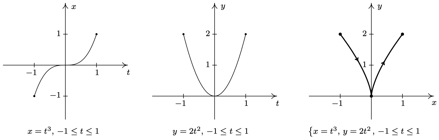
1. $\left\{\begin{array}{l} x=t^{3} \\ y=2 t^{2} \end{array} \quad \text { for }-1 \leq t \leq 1\right.$
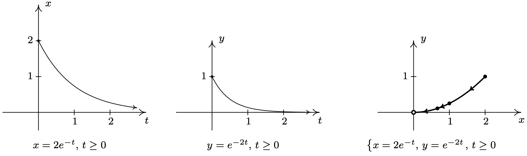
2. $\left\{\begin{array}{l} x=e^{-t} \\ y=e^{-2 t} \quad \text { for } t \geq 0 \end{array}\right.$
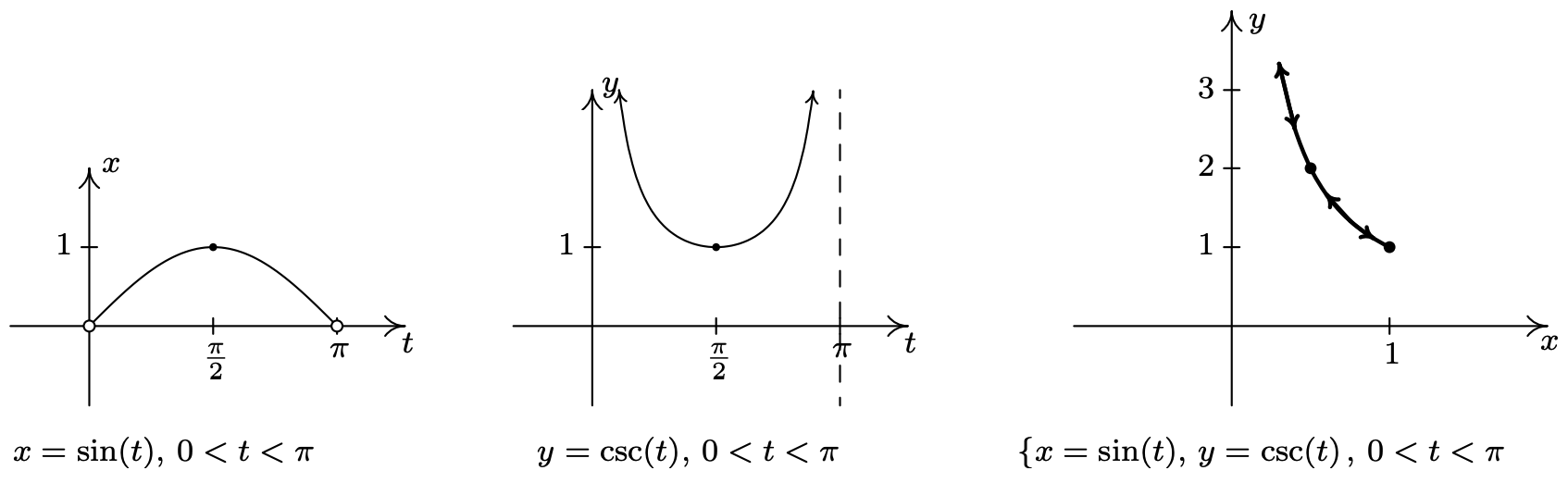
3. $\left\{\begin{array}{l} x=\sin (t) \\ y=\csc (t) \end{array} \quad \text { for } 0<t<\pi\right.$
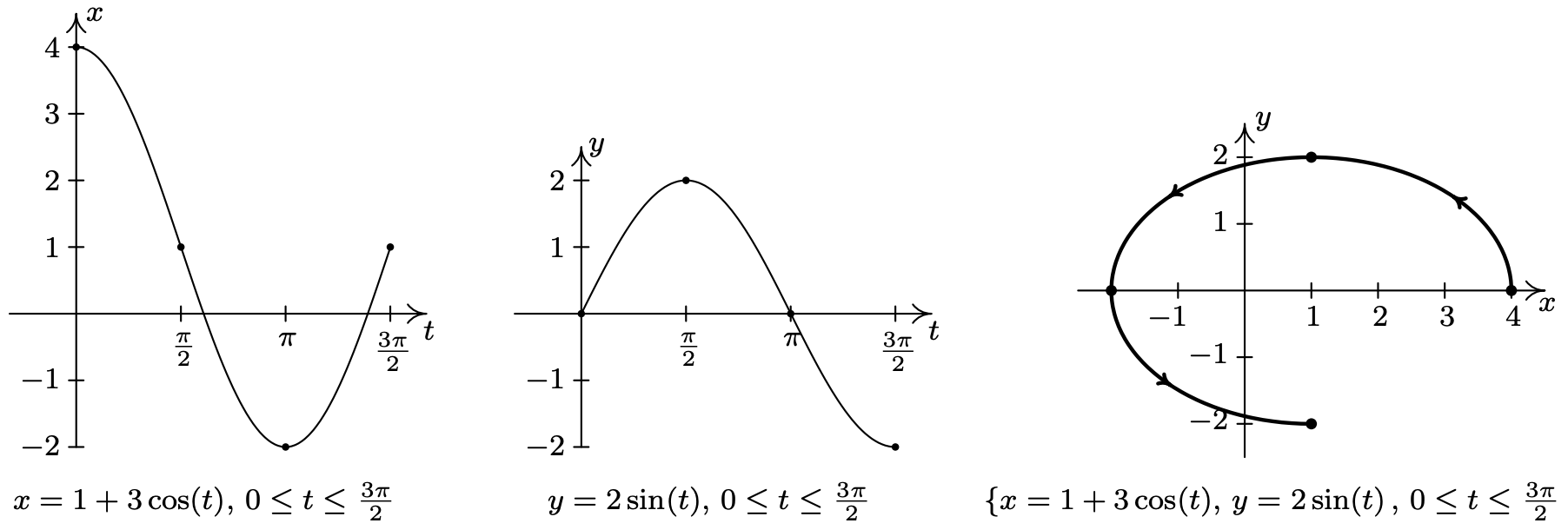
4. $\left\{\begin{array}{l} x=1+3 \cos (t) \\ y=2 \sin (t) \end{array} \quad \text { for } 0 \leq t \leq \frac{3 \pi}{2}\right.$

Solution

1. To get a feel for the curve described by the system $\left\{x=t^{3}, y=2 t^{2}\right.$ we first sketch the graphs of $x=t^{3}$ and $y=2 t^{2}$ over the interval [−1, 1]. We note that as $t$ takes on values in the interval [−1, 1], $x=t^{3}$ ranges between −1 and 1, and $y=2 t^{2}$ ranges between 0 and 2. This means that all of the action is happening on a portion of the plane, namely $\{(x, y) \mid-1 \leq x \leq 1,0 \leq y \leq 2\}$. Next, we plot a few points to get a sense of the position and orientation of the curve. Certainly, $t = −1$ and $t = 1$ are good values to pick since these are the extreme values of $t$. We also choose $t = 0$, since that corresponds to a relative minimum⁴ on the graph of $y=2 t^{2}$. Plugging in $t = −1$ gives the point (−1, 2), $t = 0$ gives (0, 0) and $t = 1$ gives (1, 2). More generally, we see that $x=t^{3}$ is increasing over the entire interval [−1, 1] whereas $y=2 t^{2}$ is decreasing over the interval [−1, 0] and then increasing over [0, 1]. Geometrically, this means that in order to trace out the path described by the parametric equations, we start at (−1, 2) (where $t = −1$), then move to the right (since $x$ is increasing) and down (since $y$ is decreasing) to (0, 0) (where $t = 0$). We continue to move to the right (since $x$ is still increasing) but now move upwards (since $y$ is now increasing) until we reach (1, 2) (where $t = 1$). Finally, to get a good sense of the shape of the curve, we eliminate the parameter. Solving $x=t^{3}$ for $t$, we get $t=\sqrt[3]{x}$. Substituting this into $y=2 t^{2}$ gives $y=2(\sqrt[3]{x})^{2}=2 x^{2 / 3}$. Our experience in Section 5.3 yields the graph of our final answer below.

   

2. For the system $\left\{x=2 e^{-t}, y=e^{-2 t} \text { for } t \geq 0\right.$, we proceed as in the previous example and graph $x=2 e^{-t}$ and $y=e^{-2 t}$ over the interval $[0, \infty)$. We find that the range of $x$ in this case is (0, 2] and the range of $y$ is (0, 1]. Next, we plug in some friendly values of $t$ to get a sense of the orientation of the curve. Since $t$ lies in the exponent here, ‘friendly’ values of $t$ involve natural logarithms. Starting with $t=\ln (1)=0$ we get⁵ (2, 1), for $t=\ln (2)$ we get $\left(1, \frac{1}{4}\right)$ and for $t=\ln (3)$ we get \left(\frac{2}{3}, \frac{1}{9}\right)\). Since $t$ is ranging over the unbounded interval $[0, \infty)$, we take the time to analyze the end behavior of both $x$ and $y$. As $t \rightarrow \infty, x=2 e^{-t} \rightarrow 0^{+}$ and $y=e^{-2 t} \rightarrow 0^{+}$ as well. This means the graph of $\left\{x=2 e^{-t}, y=e^{-2 t}\right.$ approaches the point (0, 0). Since both $x=2 e^{-t}$ and $y=e^{-2 t}$ are always decreasing for $t \geq 0$, we know that our final graph will start at (2, 1) (where $t = 0$), and move consistently to the left (since $x$ is decreasing) and down (since $y$ is decreasing) to approach the origin. To eliminate the parameter, one way to proceed is to solve $x=2 e^{-t}$ for $t$ to get $t=-\ln \left(\frac{x}{2}\right)$. Substituting this for $t$ in $y=e^{-2 t}$ gives $y=e^{-2(-\ln (x / 2))}=e^{2 \ln (x / 2)}=e^{\ln (x / 2)^{2}}=\left(\frac{x}{2}\right)^{2}=\frac{x^{2}}{4}$. Or, we could recognize that $y=e^{-2 t}=\left(e^{-t}\right)^{2}$, and since $x=2 e^{-t}$ means $e^{-t}=\frac{x}{2}$, we get $y=\left(\frac{x}{2}\right)^{2}=\frac{x^{2}}{4}$ this way as well. Either way, the graph of $\left\{x=2 e^{-t}, y=e^{-2 t} \text { for } t \geq 0\right.$ is a portion of the parabola $y=\frac{x^{2}}{4}$ which starts at the point (2, 1) and heads towards, but never reaches,⁶ (0,0).

   

3. For the system $\{x=\sin (t), y=\csc (t) \text { for } 0<t<\pi$, we start by graphing $x=\sin (t)$ and $y=\csc (t)$ over the interval $(0, \pi)$. We find that the range of $x$ is (0, 1] while the range of $y$ is $[1, \infty)$. Plotting a few friendly points, we see that $t=\frac{\pi}{6}$ gives the point $\left(\frac{1}{2}, 2\right), t=\frac{\pi}{2}$ gives (1,1) and $t=\frac{5 \pi}{6}$ return us to $\left(\frac{1}{2}, 2\right)$. Since $t=0$ and $t=\pi$ aren’t included in the domain for $t$, (because $y=\csc (t)$ is undefined at these $t$-values), we analyze the behavior of the system as $t$ approach 0 and $\pi$. We find that as $t \rightarrow 0^{+}$ as well as when $t \rightarrow \pi^{-}$, we get $x=\sin (t) \rightarrow 0^{+}$ and $y=\csc (t) \rightarrow \infty$. Piecing all of this information together, we get that for $t$ near 0, we have points with very small positive $x$-values, but very large positive $y$-values. As $t$ ranges through the through the interval $\left(0, \frac{\pi}{2}\right], x=\sin (t)$ is increasing and $y=\csc (t)$ is decreasing. This means that we are moving to the right and downwards, through $\left(\frac{1}{2}, 2\right)$ when $t=\frac{\pi}{6}$ to (1,1) when $t=\frac{\pi}{2}$. Once $t=\frac{\pi}{2}$, the orientation reverses, and we start to head to the left, since $x=\sin (t)$ is now decreasing, and up, since $y=\csc (t)$ is now increasing. We pass back through $\left(\frac{1}{2}, 2\right)$ when $t=\frac{5 \pi}{6}$ back to the points with small positive $x$-coordinates and large positive $y$-coordinates. To better explain this behavior, we eliminate the parameter. Using a reciprocal identity, we write $y=\csc (t)=\frac{1}{\sin (t)}$. Since $x=\sin (t)$, the curve traced out by this parametrization is a portion of the graph of $y=\frac{1}{x}$. We now can explain the unusual behavior as $t \rightarrow 0^{+}$ and $t \rightarrow \pi^{-}$ – for these values of $t$, we are hugging the vertical asymptote $x = 0$ of the graph of $y=\frac{1}{x}$. We see that the parametrization given above traces out the portion of $y=\frac{1}{x}$ for $0<x \leq 1$ twice as $t$ runs through the interval $(0, \pi)$.

   

4. Proceeding as above, we set about graphing $\left\{x=1+3 \cos (t), y=2 \sin (t) \text { for } 0 \leq t \leq \frac{3 \pi}{2}\right.$ by first graphing $x=1+3 \cos (t)$ and $y=2 \sin (t)$ on the interval $\left[0, \frac{3 \pi}{2}\right]$. We see that $x$ ranges from −2 to 4 and $y$ ranges from −2 to 2. Plugging in $t=0, \frac{\pi}{2}, \pi \text { and } \frac{3 \pi}{2}$ gives the points (4, 0), (1, 2), (−2, 0) and (1, −2), respectively. As $t$ ranges from 0 to $\frac{\pi}{2}, x=1+3 \cos (t)$ is decreasing, while $y=2 \sin (t)$ is increasing. This means that we start tracing out our answer at (4, 0) and continue moving to the left and upwards towards (1, 2). For $\frac{\pi}{2} \leq t \leq \pi$, $x$ is decreasing, as is $y$, so the motion is still right to left, but now is downwards from (1, 2) to (−2, 0). On the interval $\left[\pi, \frac{3 \pi}{2}\right]$, $x$ begins to increase, while $y$ continues to decrease. Hence, the motion becomes left to right but continues downwards, connecting (−2, 0) to (1, −2). To eliminate the parameter here, we note that the trigonometric functions involved, namely $\cos (t)$ and $\sin (t)$, are related by the Pythagorean Identity $\cos ^{2}(t)+\sin ^{2}(t)=1$. Hence, we solve $x=1+3 \cos (t)$ for $\cos (t)$ to get $\cos (t)=\frac{x-1}{3}$, and we solve $y=2 \sin (t)$ for $\sin (t)$ to get $\sin (t)=\frac{y}{2}$. Substituting these expressions into $\cos ^{2}(t)+\sin ^{2}(t)=1$ gives $\left(\frac{x-1}{3}\right)^{2}+\left(\frac{y}{2}\right)^{2}=1, \text { or } \frac{(x-1)^{2}}{9}+\frac{y^{2}}{4}=1$. From Section 7.4, we know that the graph of this equation is an ellipse centered at (1, 0) with vertices at (−2, 0) and (4, 0) with a minor axis of length 4. Our parametric equations here are tracing out three-quarters of this ellipse, in a counter-clockwise direction.

   

Now that we have had some good practice sketching the graphs of parametric equations, we turn to the problem of finding parametric representations of curves. We start with the following.

Parametrizations of Common Curves

• To parametrize $y = f(x)$ as $x$ runs through some interval $I$, let $x = t$ and $y = f(t)$ and let $t$ run through $I$.
• To parametrize $x = g(y)$ as $y$ runs through some interval $I$, let $x = g(t)$ and $y = t$ and let $t$ run through $I$.
• To parametrize a directed line segment with initial point $\left(x_{0}, y_{0}\right)$ and terminal point $\left(x_{1}, y_{1}\right)$, let $x=x_{0}+\left(x_{1}-x_{0}\right) t$ and $y=y_{0}+\left(y_{1}-y_{0}\right) t$ for $0 \leq t \leq 1$.
• To parametrize $\frac{(x-h)^{2}}{a^{2}}+\frac{(y-k)^{2}}{b^{2}}=1$ where $a, b > 0$, let $x=h+a \cos (t)$ and $y=k+b \sin (t)$ for $0 \leq t<2 \pi$. (This will impart a counter-clockwise orientation.)

The reader is encouraged to verify the above formulas by eliminating the parameter and, when indicated, checking the orientation. We put these formulas to good use in the following example.

Example 11.10.3

Find a parametrization for each of the following curves and check your answers.

1. $y=x^{2} \text { from } x=-3 \text { to } x=2$
2. $y=f^{-1}(x) \text { where } f(x)=x^{5}+2 x+1$
3. The line segment which starts at (2, −3) and ends at (1, 5)
4. The circle $x^{2}+2 x+y^{2}-4 y=4$
5. The left half of the ellipse $\frac{x^{2}}{4}+\frac{y^{2}}{9}=1$

Solution

1. Since $y=x^{2}$ is written in the form $y=f(x)$, we let $x = t$ and $y=f(t)=t^{2}$. Since $x = t$, the bounds on $t$ match precisely the bounds on $x$ so we get $\left\{x=t, y=t^{2} \text { for }-3 \leq t \leq 2\right.$. The check is almost trivial; with $x = t$ we have $y=t^{2}=x^{2}$ as $t = x$ runs from −3 to 2.
2. We are told to parametrize $y=f^{-1}(x)$ for $f(x)=x^{5}+2 x+1$ so it is safe to assume that $f$ is one-to-one. (Otherwise, $f^{-1}$ would not exist.) To find a formula $y=f^{-1}(x)$, we follow the procedure outlined on page 384 – we start with the equation $y = f(x)$, interchange $x$ and $y$ and solve for $y$. Doing so gives us the equation $x=y^{5}+2 y+1$. While we could attempt to solve this equation for $y$, we don’t need to. We can parametrize $x=f(y)=y^{5}+2 y+1$ by setting $y = t$ so that $x=t^{5}+2 t+1$. We know from our work in Section 3.1 that since $f(x)=x^{5}+2 x+1$ is an odd-degree polynomial, the range of $y=f(x)=x^{5}+2 x+1$ is $(-\infty, \infty)$. Hence, in order to trace out the entire graph of $x=f(y)=y^{5}+2 y+1$, we need to let $y$ run through all real numbers. Our final answer to this problem is $\left\{x=t^{5}+2 t+1, y=t\right.$ for $-\infty<t<\infty$. As in the previous problem, our solution is trivial to check.⁷
3. To parametrize line segment which starts at (2, −3) and ends at (1, 5), we make use of the formulas $x=x_{0}+\left(x_{1}-x_{0}\right) t$ and $y=y_{0}+\left(y_{1}-y_{0}\right) t$ for $0 \leq t \leq 1$. While these equations at first glance are quite a handful,⁸ they can be summarized as ‘starting point + (displacement)$t$’. To find the equation for $x$, we have that the line segment starts at $x = 2$ and ends at $x = 1$. This means the displacement in the $x$-direction is (1 − 2) = −1. Hence, the equation for $x$ is $x = 2 + (−1)t = 2 − t$. For $y$, we note that the line segment starts at $y = −3$ and ends at $y = 5$. Hence, the displacement in the $y$-direction is $(5 − (−3)) = 8$, so we get $y = −3 + 8t$. Our final answer is $\{x=2-t, y=-3+8 t$ for $0 \leq t \leq 1$. To check, we can solve $x = 2 − t$ for $t$ to get $t = 2 − x$. Substituting this into $y = −3 + 8t$ gives $y = −3 + 8t = −3 + 8(2 − x)$, or $y = −8x + 13. We know this is the graph of a line, so all we need to check is that it starts and stops at the correct points. When \(t = 0, x = 2 − t = 2$, and when $t = 1, x = 2 − t = 1$. Plugging in $x = 2$ gives $y = −8(2) + 13 = −3$, for an initial point of $(2, −3)$. Plugging in $x = 1$ gives $y = −8(1) + 13 = 5$ for an ending point of $(1, 5)$, as required.
4. In order to use the formulas above to parametrize the circle $x^{2}+2 x+y^{2}-4 y=4$, we first need to put it into the correct form. After completing the squares, we get $(x+1)^{2}+(y-2)^{2}=9$, or $\frac{(x+1)^{2}}{9}+\frac{(y-2)^{2}}{9}=1$. Once again, the formulas $x=h+a \cos (t)$ and $y=k+b \sin (t)$ can be a challenge to memorize, but they come from the Pythagorean Identity $\cos ^{2}(t)+\sin ^{2}(t)=1$. In the equation $\frac{(x+1)^{2}}{9}+\frac{(y-2)^{2}}{9}=1$, we identify $\cos (t)=\frac{x+1}{3}$ and $\sin (t)=\frac{y-2}{3}$. Rearranging these last two equations, we get $x=-1+3 \cos (t)$ and $y=2+3 \sin (t)$. In order to complete one revolution around the circle, we let $t$ range through the interval $[0,2 \pi)$. We get as our final answer $\{x=-1+3 \cos (t), y=2+3 \sin (t)$ for $0 \leq t<2 \pi$. To check our answer, we could eliminate the parameter by solving $x=-1+3 \cos (t)$ for $\cos (t)$ and $y=2+3 \sin (t)$ for $\sin (t)$, invoking a Pythagorean Identity, and then manipulating the resulting equation in $x$ and $y$ into the original equation $x^{2}+2 x+y^{2}-4 y=4$. Instead, we opt for a more direct approach. We substitute $x=-1+3 \cos (t)$ and $y=2+3 \sin (t)$ into the equation $x^{2}+2 x+y^{2}-4 y=4$ and show that the latter is satisfied for all $t$ such that $0 \leq t<2 \pi$. $$\begin{array}{rlll} x^{2}+2 x+y^{2}-4 y & = & 4 \\ (-1+3 \cos (t))^{2}+2(-1+3 \cos (t))+(2+3 \sin (t))^{2}-4(2+3 \sin (t)) & \stackrel{?}{=} & 4 \\ 1-6 \cos (t)+9 \cos ^{2}(t)-2+6 \cos (t)+4+12 \sin (t)+9 \sin ^{2}(t)-8-12 \sin (t) & \stackrel{?}{=} & 4 \\ 9 \cos ^{2}(t)+9 \sin ^{2}(t)-5 & \stackrel{?}{=} & 4 \\ 9\left(\cos ^{2}(t)+\sin ^{2}(t)\right)-5 & \stackrel{?}{=} & 4 \\ 9(1) -5 & \stackrel{?}{=} & 4 \\ 4 &\stackrel{\checkmark}{=} & 4 \end{array}\nonumber$$ Now that we know the parametric equations give us points on the circle, we can go through the usual analysis as demonstrated in Example 11.10.2 to show that the entire circle is covered as $t$ ranges through the interval $[0,2 \pi)$.
5. In the equation $\frac{x^{2}}{4}+\frac{y^{2}}{9}=1$, we can either use the formulas above or think back to the Pythagorean Identity to get $x=2 \cos (t)$ and $y=3 \sin (t)$. The normal range on the parameter in this case is $0 \leq t<2 \pi$, but since we are interested in only the left half of the ellipse, we restrict $t$ to the values which correspond to Quadrant II and Quadrant III angles, namely $\frac{\pi}{2} \leq t \leq \frac{3 \pi}{2}$. Our final answer is $\{x=2 \cos (t), y=3 \sin (t)$ for $\frac{\pi}{2} \leq t \leq \frac{3 \pi}{2}$. Substituting $x=2 \cos (t)$ and $y=3 \sin (t)$ into $\frac{x^{2}}{4}+\frac{y^{2}}{9}=1$ gives $\frac{4 \cos ^{2}(t)}{4}+\frac{9 \sin ^{2}(t)}{9}=1$, which reduces to the Pythagorean Identity $\cos ^{2}(t)+\sin ^{2}(t)=1$. This proves that the points generated by the parametric equations $\{x=2 \cos (t), y=3 \sin (t)$ lie on the ellipse $\frac{x^{2}}{4}+\frac{y^{2}}{9}=1$. Employing the techniques demonstrated in Example 11.10.2, we find that the restriction $\frac{\pi}{2} \leq t \leq \frac{3 \pi}{2}$ generates the left half of the ellipse, as required.

We note that the formulas given on page 1053 offer only one of literally infinitely many ways to parametrize the common curves listed there. At times, the formulas offered there need to be altered to suit the situation. Two easy ways to alter parametrizations are given below.

Adjusting Parametric Equations

• Reversing Orientation: Replacing every occurrence of $t$ with $−t$ in a parametric description for a curve (including any inequalities which describe the bounds on $t$) reverses the orientation of the curve.
• Shift of Parameter: Replacing every occurrence of $t$ with $(t − c)$ in a parametric description for a curve (including any inequalities which describe the bounds on $t$) shifts the start of the parameter $t$ ahead by $c$ units.

We demonstrate these techniques in the following example.

Example 11.10.4

Find a parametrization for the following curves.

1. The curve which starts at (2, 4) and follows the parabola $y=x^{2}$ to end at (−1, 1). Shift the parameter so that the path starts at $t = 0$.
2. The two part path which starts at (0, 0), travels along a line to (3, 4), then travels along a line to (5, 0).
3. The Unit Circle, oriented clockwise, with $t = 0$ corresponding to (0, −1).

Solution

1. We can parametrize $y=x^{2}$ from $x = −1$ to $x = 2$ using the formula given on Page 1053 as $\left\{x=t, y=t^{2}\right.$ for $-1 \leq t \leq 2$. This parametrization, however, starts at (−1, 1) and ends at (2, 4). Hence, we need to reverse the orientation. To do so, we replace every occurrence of $t$ with $−t$ to get $\left\{x=-t, y=(-t)^{2}\right.$ for $-1 \leq-t \leq 2$. After simplifying, we get $\left\{x=-t, y=t^{2}\right.$ for $-2 \leq t \leq 1$. We would like $t$ to begin at $t = 0$ instead of $t = −2$. The problem here is that the parametrization we have starts 2 units ‘too soon’, so we need to introduce a ‘time delay’ of 2. Replacing every occurrence of $t$ with $(t-2)$ gives $\left\{x=-(t-2), y=(t-2)^{2}\right.$ for $-2 \leq t-2 \leq 1$. Simplifying yields $\left\{x=2-t, y=t^{2}-4 t+4 \text { for } 0 \leq t \leq 3\right.$.
2. When parameterizing line segments, we think: ‘starting point + (displacement)$t$’. For the first part of the path, we get $\{x=3 t, y=4 t$ for $0 \leq t \leq 1$, and for the second part we get $\{x=3+2 t, y=4-4 t$ for $0 \leq t \leq 1$. Since the first parametrization leaves off at $t = 1$, we shift the parameter in the second part so it starts at $t = 1$. Our current description of the second part starts at $t = 0$, so we introduce a ‘time delay’ of 1 unit to the second set of parametric equations. Replacing $t$ with $(t − 1)$ in the second set of parametric equations gives $\{x=3+2(t-1), y=4-4(t-1)$ for $0 \leq t-1 \leq 1$. Simplifying yields $\{x=1+2 t, y=8-4 t$ for $1 \leq t \leq 2$. Hence, we may parametrize the path as $\{x=f(t), y=g(t)$ for $0 \leq t \leq 2$ where $$f(t)=\left\{\begin{aligned} 3 t, & \text { for } 0 \leq t \leq 1 \\ 1+2 t, & \text { for } 1 \leq t \leq 2 \end{aligned} \quad \text { and } \quad g(t)=\left\{\begin{aligned} 4 t, & \text { for } 0 \leq t \leq 1 \\ 8-4 t, & \text { for } 1 \leq t \leq 2 \end{aligned}\right.\right.\nonumber$$
3. We know that $\{x=\cos (t), y=\sin (t)$ for $0 \leq t<2 \pi$ gives a counter-clockwise parametrization of the Unit Circle with $t = 0$ corresponding to (1, 0), so the first order of business is to reverse the orientation. Replacing $t$ with $−t$ gives $\{x=\cos (-t), y=\sin (-t)$ for $0 \leq-t<2 \pi$, which simplifies⁹ to $\{x=\cos (t), y=-\sin (t)$ for $-2 \pi<t \leq 0$. This parametrization gives a clockwise orientation, but $t = 0$ still corresponds to the point (1, 0); the point (0, −1) is reached when $t=-\frac{3 \pi}{2}$. Our strategy is to first get the parametrization to ‘start’ at the point (0, −1) and then shift the parameter accordingly so the ‘start’ coincides with $t = 0$. We know that any interval of length $2\pi$ will parametrize the entire circle, so we keep the equations $\{x=\cos (t), y=-\sin (t)$, but start the parameter $t$ at $-\frac{3 \pi}{2}$, and find the upper bound by adding $2\pi$ so $-\frac{3 \pi}{2} \leq t<\frac{\pi}{2}$. The reader can verify that $\{x=\cos (t), y=-\sin (t)$ for $-\frac{3 \pi}{2} \leq t<\frac{\pi}{2}$ traces out the Unit Circle clockwise starting at the point (0, −1). We now shift the parameter by introducing a ‘time delay’ of $\frac{3 \pi}{2}$ units by replacing every occurrence of $t$ with $\left(t-\frac{3 \pi}{2}\right)$. We get $\left\{x=\cos \left(t-\frac{3 \pi}{2}\right), y=-\sin \left(t-\frac{3 \pi}{2}\right)\right.$ for $-\frac{3 \pi}{2} \leq t-\frac{3 \pi}{2}<\frac{\pi}{2}$. This simplifies¹⁰ to $\{x=-\sin (t), y=-\cos (t)$ for $0 \leq t<2 \pi$, as required.

We put our answer to Example 11.10.4 number 3 to good use to derive the equation of a cycloid. Suppose a circle of radius $r$ rolls along the positive $x$-axis at a constant velocity $v$ as pictured below. Let $\theta$ be the angle in radians which measures the amount of clockwise rotation experienced by the radius highlighted in the figure.

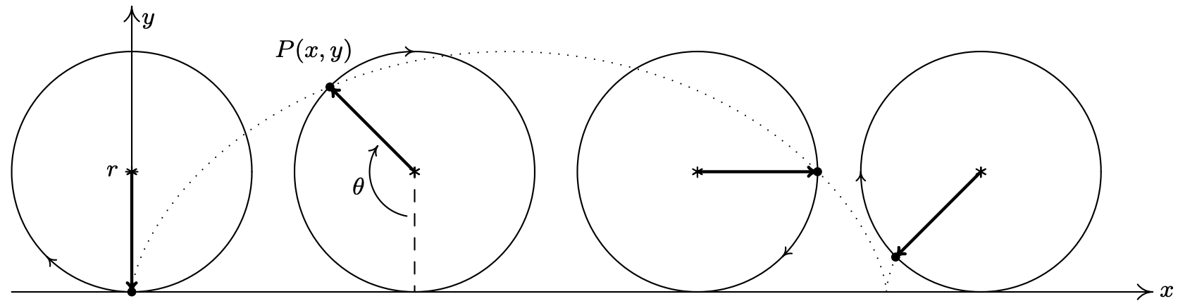
Our goal is to find parametric equations for the coordinates of the point $P(x, y)$ in terms of $\theta$. From our work in Example 11.10.4 number 3, we know that clockwise motion along the Unit Circle starting at the point (0, −1) can be modeled by the equations $\{x=-\sin (\theta), y=-\cos (\theta)$ for $0 \leq \theta<2 \pi$. (We have renamed the parameter '$\theta$' to match the context of this problem.) To model this motion on a circle of radius $r$, all we need to do¹¹ is multiply both $x$ and $y$ by the factor $r$ which yields $\{x=-r \sin (\theta), y=-r \cos (\theta)$. We now need to adjust for the fact that the circle isn’t stationary with center (0, 0), but rather, is rolling along the positive $x$-axis. Since the velocity $v$ is constant, we know that at time $t$, the center of the circle has traveled a distance $vt$ down the positive $x$-axis. Furthermore, since the radius of the circle is $r$ and the circle isn’t moving vertically, we know that the center of the circle is always $r$ units above the $x$-axis. Putting these two facts together, we have that at time $t$, the center of the circle is at the point $(vt, r)$. From Section 10.1.1, we know $v=\frac{r \theta}{t}$, or $v t=r \theta$. Hence, the center of the circle, in terms of the parameter $\theta$, is $(r \theta, r)$. As a result, we need to modify the equations $\{x=-r \sin (\theta), y=-r \cos (\theta)$ by shifting the $x$-coordinate to the right $r \theta$ units (by adding $r \theta$ to the expression for $x$) and the $y$-coordinate up $r$ units¹² (by adding $r$ to the expression for $y$). We get $\{x=-r \sin (\theta)+r \theta, y=-r \cos (\theta)+r$, which can be written as $\{x=r(\theta-\sin (\theta)), y=r(1-\cos (\theta))$. Since the motion starts at $\theta=0$ and proceeds indefinitely, we set $\theta \geq 0$.

We end the section with a demonstration of the graphing calculator.

Example 11.10.5

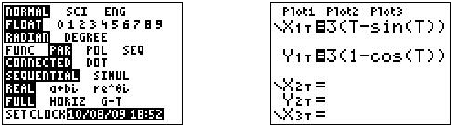
Find the parametric equations of a cycloid which results from a circle of radius 3 rolling down the positive $x$-axis as described above. Graph your answer using a calculator.

Solution

We have $r = 3$ which gives the equations $\{x=3(t-\sin (t)), y=3(1-\cos (t))$ for $t \geq 0$. (Here we have returned to the convention of using $t$ as the parameter.) Sketching the cycloid by hand is a wonderful exercise in Calculus, but for the purposes of this book, we use a graphing utility. Using a calculator to graph parametric equations is very similar to graphing polar equations on a calculator.¹³ Ensuring that the calculator is in ‘Parametric Mode’ and ‘radian mode’ we enter the equations and advance to the ‘Window’ screen.

As always, the challenge is to determine appropriate bounds on the parameter, $t$, as well as for $x$ and $y$. We know that one full revolution of the circle occurs over the interval $0 \leq t<2 \pi$, so it seems reasonable to keep these as our bounds on $t$. The ‘Tstep’ seems reasonably small – too large a value here can lead to incorrect graphs.¹⁴ We know from our derivation of the equations of the cycloid that the center of the generating circle has coordinates $(r \theta, r)$, or in this case, $(3 t, 3)$. Since $t$ ranges between 0 and $2 \pi$, we set $x$ to range between 0 and $6 \pi$. The values of $y$ go from the bottom of the circle to the top, so $y$ ranges between 0 and 6.

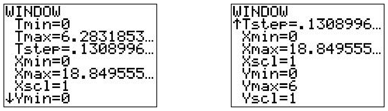
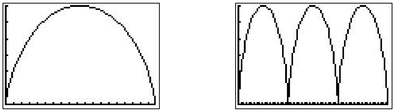
Below we graph the cycloid with these settings, and then extend $t$ to range from 0 to $6\pi$ which forces $x$ to range from 0 to $18\pi$ yielding three arches of the cycloid. (It is instructive to note that keeping the $y$ settings between 0 and 6 messes up the geometry of the cycloid. The reader is invited to use the Zoom Square feature on the graphing calculator to see what window gives a true geometric perspective of the three arches.)

¹ Note the use of the indefinite article ‘a’. As we shall see, there are infinitely many different parametric representations for any given curve.

² Here, the bug reaches the point $Q$ at two different times. While this does not contradict our claim that $f(t)$ and $g(t)$ are functions of $t$, it shows that neither $f$ nor $g$ can be one-to-one. (Think about this before reading on.)

³ We will have an example shortly where no matter how we restrict x and y, we can never accurately describe the curve once we’ve eliminated the parameter.

⁴ You should review Section 1.6.1 if you’ve forgotten what ‘increasing’, ‘decreasing’ and ‘relative minimum’ mean.

⁵ The reader is encouraged to review Sections 6.1 and 6.2 as needed.

⁶ Note the open circle at the origin. See the solution to part 3 in Example 1.2.1 on page 22 and Theorem 4.1 in Section 4.1 for a review of this concept.

⁷ Provided you followed the inverse function theory, of course.

⁸ Compare and contrast this with Exercise 65 in Section 11.8.

⁹ courtesy of the Even/Odd Identities

¹⁰ courtesy of the Sum/Difference Formulas

¹¹ If we replace $x$ with $\frac{x}{r}$ and $y$ with $\frac{y}{r}$ in the equation for the Unit Circle $x^{2}+y^{2}=1$, we obtain $\left(\frac{x}{r}\right)^{2}+\left(\frac{y}{r}\right)^{2}=1$ which reduces to $x^{2}+y^{2}=r^{2}$. In the language of Section 1.7, we are stretching the graph by a factor of $r$ in both the $x$- and $y$-directions. Hence, we multiply both the $x$- and $y$-coordinates of points on the graph by $r$.

¹² Does this seem familiar? See Example 11.1.1 in Section 11.1.

¹³ See page 959 in Section 11.5.

¹⁴ Again, see page 959 in Section 11.5.

¹⁵ A nice mix of vectors and Calculus are needed to derive this.

¹⁶ We’ve seen this before. It’s the angle of elevation which was defined on page 753.