4.4: Polynomial Division

Learning Objectives

• Divide polynomials using long division
• Divide polynomials using synthetic division
• Apply the factor and remainder theorems to polynomials

Are You Ready?

Try these questions prior to beginning this section to help determine if you are set up for success:

1. Simplify the expression:
   1. \(\quad (4x^2+2x+1)(x-4)+1\)
   2. \(\quad \dfrac{15z^4-18z^3+24z^2-9z}{3z}\)

Answer

1. 1. \(\quad 4x^3-14x^2-7x-3\)
   2. \(\quad 5z^3-6z^2+8z-3\)

If you missed this problem or feel you could use more practice, review [ 2.6: Multiplying Polynomial Expressions and 2.13: Simplifying, Multiplying, and Dividing Rational Expressions]

Suppose we wish to find the x-intercepts of \(f(x) = x^3 + 4x^2-5x-14\). Setting \(f(x)=0\) results in the polynomial equation \(x^3 + 4x^2-5x-14=0\). Despite all of the factoring techniques we learned in Intermediate Algebra courses, this equation foils us at every turn since these factoring techniques do no work. If we graph \(f\) using a graphing calculator window [-5,5]x[-16,16], we get

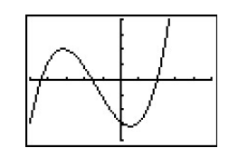
The graph suggests that the function has three x-intercepts, one of which is at \(x=2\). It's easy to show that \(f(2) = 0\), but the other two x-intercepts seem to be less friendly. Even though we could use the 'Zero' command to find decimal approximations for these x-intercepts, we seek a method to find the exact values of the other x-intercepts. Based on our experience in the previous section, if there is an x-intercept at \(x=2\), it seems that there should be a factor of \((x-2)\) for \(f(x)\). In other words, we should expect that \(x^3 + 4x^2-5x-14=(x-2) \, q(x)\), where \(q(x)\) is some other polynomial. How could we find such a \(q(x)\), if it even exists? The answer comes from our old friend, division.

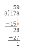
We are familiar with long division from ordinary arithmetic. We begin by dividing into the digits of the dividend that have the greatest place value. We divide, multiply, subtract, include the digit in the next place value position, and repeat. For example, let’s divide 178 by 3 using long division.

Long Division

Step 1: \(5 \times 3=15\) and \(17-15=2\) Step 2: Bring down the 8 Step 3: \(9 \times 3=27\) and \(28-27=1\) Answer: \(59 R 1\) or \(59 \frac{1}{3}\)

Another way to look at the solution is as a sum of parts. This should look familiar, since it is the same method used to check division in elementary arithmetic.

\[\begin{align*} \text{dividend}&=(\text{divisor}{\cdot}\text{quotient})+\text{remainder} \\ 178&=(3{\cdot}59)+1 \\ &=177+1 \\ &=178\end{align*}\]

We can also state that \(\frac{178}{3}=59+\frac{1}{3}\) which is the algebraic form of the mixed number \(59\frac{1}{3}\)

We call this the Division Algorithm.

Long Division of Polynomials

Now, let's revisit the the polynomial \(f(x) = x^3 + 4x^2-5x-14\). In the last section we saw that we could write a polynomial as a product of factors, each corresponding to a x-intercept. If we know that there is an x-intercept at \(x = 2\) for \(f(x)\), then we might guess that the polynomial could be factored as \(x^{3} +4x^{2} -5x-14=(x-2)\) (something). To find that "something," we can use polynomial division.

Example \(\PageIndex{1}\)

Divide \(x^{3} +4x^{2} -5x-14\) by \(x-2\).

Solution

Start by writing the problem out in long division form

\(x - 2 \longdiv { x ^ { 3 } + 4 x ^ { 2 } - 5 x - 1 4 }\)

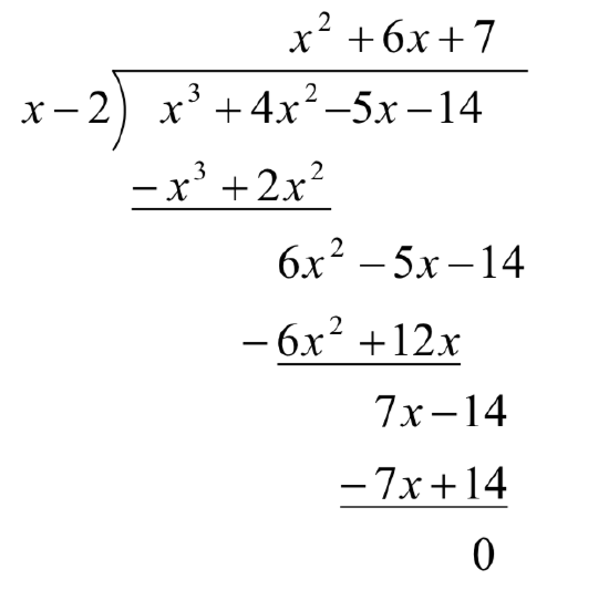
Now we divide the leading terms: \(x^{3} \div x=x^{2}\). It is best to align it above the same-powered term in the dividend. Now, multiply that \(x^{2}\) by \(x-2\) and write the result below the dividend.

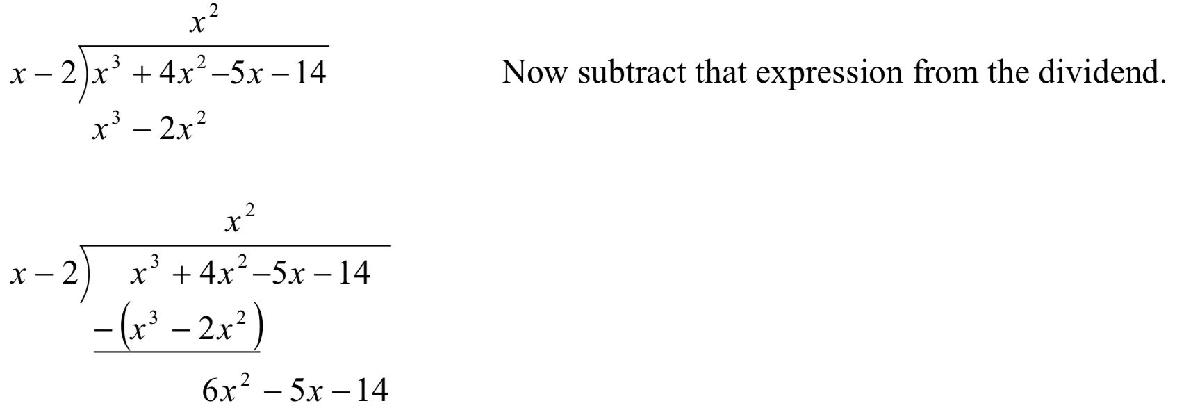
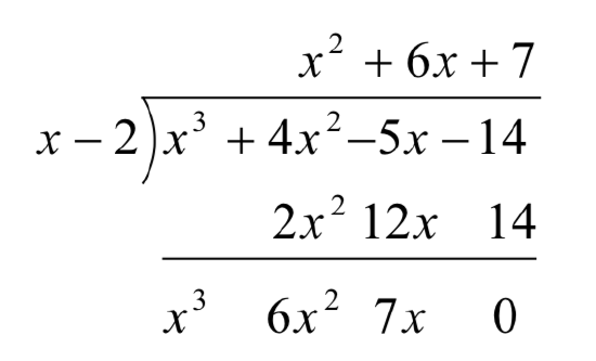
Again, divide the leading term of the remainder by the leading term of the divisor. \(6x^{2} \div x=6x\). We add this to the result, multiply 6x by \(x-2\), and subtract.

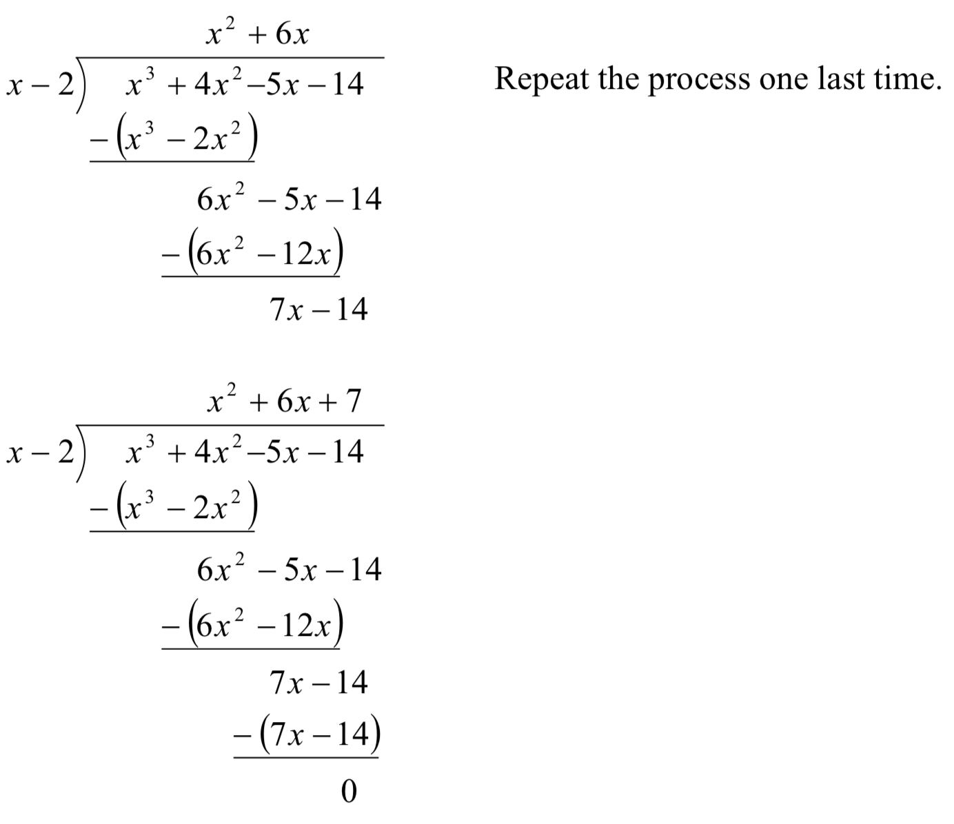
This tells us \(x^{3} +4x^{2} -5x-14\) divided by \(x-2\) is \(x^{2} +6x+7\), with a remainder of zero. This also means that we can factor \(x^{3} +4x^{2} -5x-14\) as \(\left(x-2\right)\left(x^{2} +6x+7\right)\).

Now, if we want to find the other x-intercepts, we now solve \(x^2+6x+7=0\). Since this doesn't factor nicely we can complete the square or use the Quadratic Formula to get \(x = -3 \pm \sqrt{2}\). The point of this section is to focus on how to perform division. Before looking at more examples, let's note what we can expect when we divide polynomials.

The Division Algorithm for Polynomials

Suppose \(d(x)\) and \(p(x)\) are nonzero polynomials where the degree of \(p\) is greater than or equal to the degree of \(d\). There exist two unique polynomials, \(q(x)\) and \(r(x)\), such that \[p(x) = d(x) \, q(x) + r(x),\nonumber \]

or \[\frac{p(x)}{d(x)}=q(x)+\frac{r(x)}{d(x)} \nonumber \]

where either \(r(x) = 0\) or the degree of \(r\) is strictly less than the degree of \(d\).

The polynomial \(p\) is called the dividend; \(d\) is the divisor; \(q\) is the quotient; \(r\) is the remainder. If \(r(x)=0\) then \(d\) is called a factor of \(p\).

Because of the division, the remainder will either be zero, or a polynomial of lower degree than d(x). Because of this, if we divide a polynomial by a term of the form \(x-c\), then the remainder will be zero or a constant.

If \(p(x)=(x-c)q(x)+r\), then \(p(c)=(c-c)q(c)+r=0+r=r\), which establishes the Remainder Theorem.

The Remainder Theorem

If \(p(x)\) is a polynomial of degree 1 or greater and c is a real number, then when p(x) is divided by \(x-c\), the remainder is \(p(c)\).

If \(x-c\) is a factor of the polynomial \(p\), then \(p(x)=(x-c)q(x)\) for some polynomial \(q\). Then \(p(c)=(c-c)q(c)=0\), showing \(c\) is a zero of the polynomial. This shouldn’t surprise us - we already knew that if the polynomial factors it reveals the roots.

If \(p(c)=0\), then the remainder theorem tells us that if p is divided by \(x-c\), then the remainder will be zero, which means \(x-c\) is a factor of \(p\).

The solutions to an equation \(p(x)=0\) are called zeros of \(p(x)\). Zeros can be real numbers or complex numbers. As we have seen with quadratics, real zeros corresponding to x-coordinates of x-intercepts and complex zeros do not.

The Factor Theorem

If \(p(x)\) is a nonzero polynomial, then the real number \(c\) is a zero of \(p(x)\) if and only if \(x-c\) is a factor of \(p(x)\).

Example \(\PageIndex{2}\)

Divide \(5x^2+3x−2\) by \(x+1\).

Solution

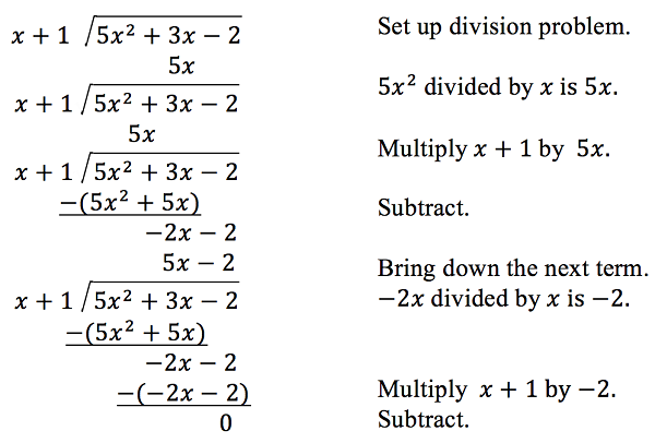
The quotient is \(5x−2\). The remainder is 0. We write the result as

\[\dfrac{5x^2+3x−2}{x+1}=5x−2\nonumber \]

Analysis

This division problem had a remainder of 0. This tells us that \((x+1)\) is a factor of \(5x^2+3x−2\), meaning \(5x^2+3x−2=(x+1)(5x−2)\), and that \(x=-1\) is a zero of \(p(x)=5x^2+3x−2\).

Example \(\PageIndex{3}\)

Divide \(6x^3+11x^2−31x+15\) by \(3x−2\).

Solution

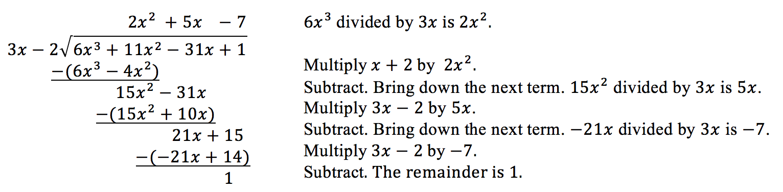
There is a remainder of 1. We can express the result as:

\[\dfrac{6x^3+11x^2−31x+15}{3x−2}=2x^2+5x−7+\dfrac{1}{3x−2}\nonumber \]

Analysis

We can check our work by using the Division Algorithm to rewrite the solution, then multiply.

\[(3x−2)(2x^2+5x−7)+1=6x^3+11x^2−31x+15\nonumber \]

Notice, as we write our result,

• the dividend is \(6x^3+11x^2−31x+15\)
• the divisor is \(3x−2\)
• the quotient is \(2x^2+5x−7\)
• the remainder is \(1\). Since the remainder is \(1\) we know that \(3x−2\) is not a factor of \(6x^3+11x^2−31x+15\).

Synthetic Division

Since dividing by \(x-c\) is a way to check if a number, \(c\), is a zero of the polynomial, it would be nice to have a faster way to divide by \(x-c\) than having to use long division every time. Happily, quicker ways have been discovered.

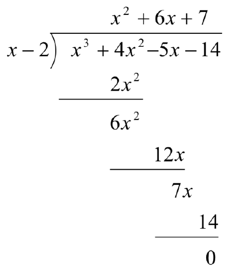
Let’s look back at the long division we did in Example 1 and try to streamline it. First, let’s distribute the negatives in the subtraction steps:

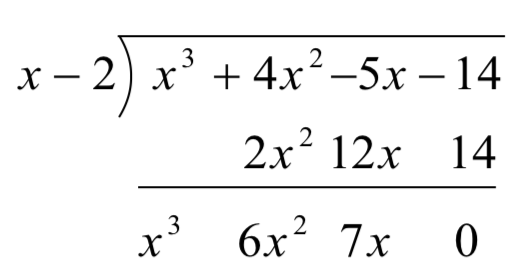
Next, observe that the terms \(-x^{3}\), \(-6x^{2}\), and \(-7x\) are the exact opposite of the terms above them. Also note that the terms we ‘bring down’ (namely the \(\mathrm{-}\)5x and \(\mathrm{-}\)14) aren’t really necessary to recopy since we know they will cancel out when we subtract, so let's omit them, too:

Now, let’s move things up a bit and, for reasons which will become clear in a moment, copy the \(x^{3}\) into the last row.

Note that by arranging things in this manner, each term in the last row is obtained by adding the two terms above it. Notice also that the quotient polynomial can be obtained by dividing each of the first three terms in the last row by \(x\) and adding the results. If you take the time to work back through the original division problem, you will find that this is exactly the way we determined the quotient polynomial.

This means that we no longer need to write the quotient polynomial down, nor the \(x\) in the divisor, to determine our answer.

We’ve streamlined things quite a bit so far, but we can still do more. Let’s take a moment to remind ourselves where the \(2x^{2}\), \(12x\) and 14 came from in the second row. Each of these terms was obtained by multiplying the terms in the quotient, \(x^{2}\), 6x and 7, respectively, by the -2 in \(x - 2\), then by -1 when we changed the subtraction to addition. Multiplying by -2 then by -1 is the same as multiplying by 2, so we replace the -2 in the divisor by 2. Furthermore, the coefficients of the quotient polynomial match the coefficients of the first three terms in the last row, so we now take the plunge and write only the coefficients of the terms to get

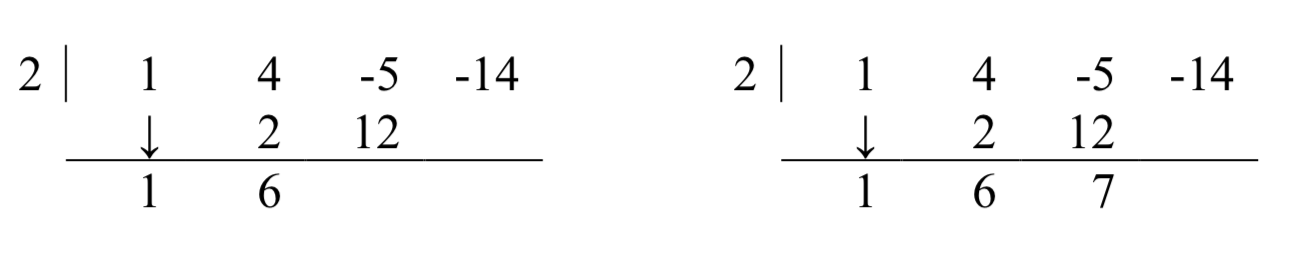
We have constructed a synthetic division tableau for this polynomial division problem. Let’s re-work our division problem using this tableau to see how it greatly streamlines the division process. To divide \(x^{3} +4x^{2} -5x-14\) by \(x-2\), we write 2 in the place of the divisor and the coefficients of \(x^{3} +4x^{2} -5x-14\) in for the dividend. Then "bring down" the first coefficient of the dividend.

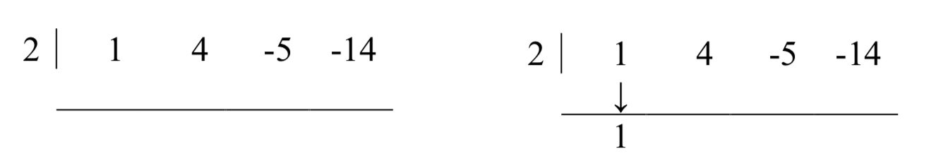
Next, take the 2 from the divisor and multiply by the 1 that was "brought down" to get 2. Write this underneath the 4, then add to get 6.

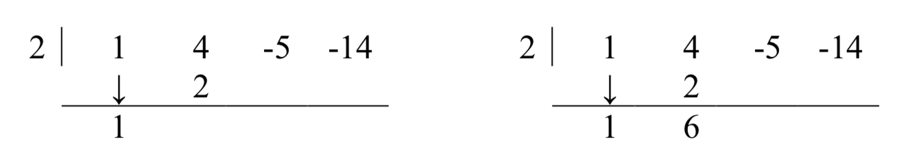
Now take the 2 from the divisor times the 6 to get 12, and add it to the -5 to get 7.

Finally, take the 2 in the divisor times the 7 to get 14, and add it to the -14 to get 0.

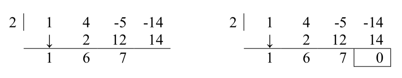
The first three numbers in the last row of our tableau are the coefficients of the quotient polynomial. Remember, we started with a third degree polynomial and divided by a first degree polynomial, so the quotient is a second degree polynomial. Hence the quotient is \(x^{2} +6x+7\). The number in the box is the remainder. Synthetic division is our tool of choice for dividing polynomials by divisors of the form \(x - c\). It is important to note that it works only for these kinds of divisors. Also take note that when a polynomial (of degree at least 1) is divided by \(x - c\), the result will be a polynomial of exactly one less degree. Finally, it is worth the time to trace each step in synthetic division back to its corresponding step in long division.

Example \(\PageIndex{4}\)

Use synthetic division to divide \(5x^{3} -2x^{2} +1\) by \(x-3\).

Solution

When setting up the synthetic division tableau, we need to enter 0 for the coefficient of \(x\) in the dividend. Doing so gives

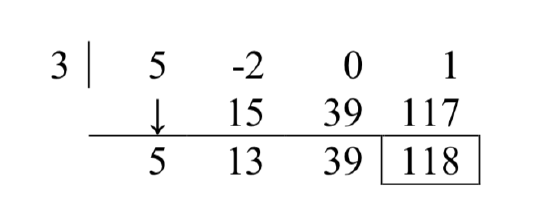
Since the dividend was a third degree polynomial, the quotient is a quadratic polynomial with coefficients 5, 13 and 39. Our quotient is \(q(x)=5x^{2} +13x+39\) and the remainder is \(r(x) = 118\). We can express this as \[\frac{5x^{3} -2x^{2} +1}{x-3}=5x^{2} +13x+39+\frac{118}{x-3}\nonumber \]

We also know that \(x-3\) is not a factor of \(5x^{3} -2x^{2} +1\) since the remainder is not zero.

Example \(\PageIndex{5}\)

Divide \(x^{3} +8\) by \(x+2\).

Solution

For this division, we rewrite \(x+2\) as \(x-\left(-2\right)\) and proceed as before.

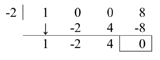
The quotient is \(x^{2} -2x+4\) and the remainder is zero. Since the remainder is zero, \(x+2\) is a factor of \(x^{3} +8\).

\[x^{3} +8=(x+2)\left(x^{2} -2x+4\right)\nonumber \]

We can write our answer as \[\dfrac{x^{3} +8}{x+2}=x^{2} -2x+4\nonumber \]

Note in the last example that there are placeholders for the missing \(x^2\) and \(x\) terms. When using synthetic division you must put place holders for the missing terms for the division to work properly.

You Try \(\PageIndex{1}\)

Divide \(4x^{4} -8x^{2} -5x\) by \(x-3\) using synthetic division.

Answer

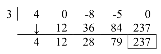
\(4x^4 - 8x^2 - 5x\) divided by \(x -3\) is \(4x^3 + 12x^2 + 28x + 79\) with remainder 237

Using this process allows us to find the real zeros of polynomials, presuming we can figure out at least one root. We’ll explore how to do that in the next section.

Example \(\PageIndex{6}\)

The polynomial \(p(x)=4x^{4} -4x^{3} -11x^{2} +12x-3\) has a horizontal intercept at \(x=\dfrac{1}{2}\) with multiplicity 2. Find the other intercepts of \(p(x)\).

Solution

Since \(x=\dfrac{1}{2}\) is an intercept with multiplicity 2, then \(x-\dfrac{1}{2}\) is a factor twice. Use synthetic division to divide by \(x-\dfrac{1}{2}\) twice.

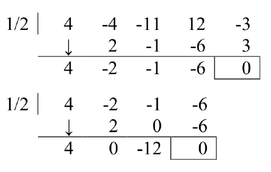
From the first division, we get \(4x^{4} -4x^{3} -11x^{2} +12x-3=\left(x-\dfrac{1}{2} \right)\left(4x^{3} -2x^{2} -x-6\right)\) The second division tells us

\[4x^{4} -4x^{3} -11x^{2} +12x-3=\left(x-\dfrac{1}{2} \right)\left(x-\dfrac{1}{2} \right)\left(4x^{2} -12\right)\nonumber \]

To find the remaining intercepts, we set \(4x^{2} -12=0\) and get \(x=\pm \sqrt{3}\).

Note this also means \(4x^{4} -4x^{3} -11x^{2} +12x-3=4\left(x-\dfrac{1}{2} \right)\left(x-\dfrac{1}{2} \right)\left(x-\sqrt{3} \right)\left(x+\sqrt{3} \right)\).

Let's summarize what we've learned about zeros and polynomial functions:

Connections Between Zeros, Factors, and Graphs of Polynomial Functions

Suppose \(p\) is a polynomial function of degree \(n \geq 1\). The following statements are equivalent:

• The real number \(c\) is a zero of \(p\)
• \(p(c) = 0\)
• \(x = c\) is a solution to the polynomial equation \(p(x) = 0\)
• \((x - c)\) is a factor of \(p(x)\)
• The point \((c, 0)\) is an \(x\)-intercept of the graph of \(y = p(x)\)