
7.4: Modeling with Exponential Functions


- Last updated
- May 4, 2022
- Save as PDF

( \newcommand{\kernel}{\mathrm{null}\,}\)
Students will be able to:
- Make predictions by using the exponential growth (or decay) model
- Use the doubling-time and half-life models to make predictions
- Estimate the doubling time and half-life by using the Rule of 70
in order to apply mathematical modeling to solve real-world applications.
The next growth we will examine is exponential growth. Linear growth occurs by adding the same amount in each unit of time. Exponential growth happens when an initial population increases by the same percentage or factor over equal time increments or generations. This is known as relative growth and is usually expressed as a percentage. For example, let’s say a population is growing by 5% each year. This means that 5% of the current population is added each year to the total. If the population was originally 10,000 in the first year, then 5% of 10,000 would be added which is 500, giving a new population of 10,500. In the second year, another 5% would be added, but this time you would take 5% of 10,500 which is 525, giving a new population of 11,025. While the percentage growth is the same each year, the actual number of people added changes, which makes this growth different from the linear model discussed earlier!
A quantity grows exponentially if it grows by a constant factor or rate for each unit of time.
In this graph, the blue straight line represents linear growth and the red curved line represents exponential growth.
A city is growing at a rate of 1.6% per year. The initial population in 2010 is P0=125,000. Calculate the city’s population over the next few years.
Solution
The relative growth rate is 1.6%. This means an additional 1.6% is added on to 100% of the population that already exists each year. This is a growth factor of 101.6%.
- Population in 2011 125,000(1.016)1=127,000
- Population in 2012 127,000(1.016)=125,000(1.016)2=129,032
- Population in 2013 129,032(1.016)=125,000(1.016)3=131,097
We can create an equation for the city’s growth. Each year the population is 101.6% more than the previous year.
P(t)=125,000(1+0.016)t
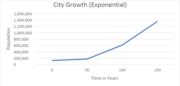
Note: The graph of the city growth follows an exponential growth model
St. Louis, Missouri has declined in population at a rate of 1.6 % per year over the last 60 years. The population in 1950 was 857,000. Find the population in 2014. (Wikipedia, n.d.)
Solution
P0=857,000
The relative rate of decrease (known as a decay rate) is 1.6%. This means 1.6% of the population is subtracted from 100% of the population that already exists each year. This is a factor of 98.4%.
- Population in 1951 857,000(0.984)1=843,288
- Population in 1952 843,228(0.984)=857,000(0.984)2=829,795
- Population in 1953 828,795(0.984)=857,000(0.984)3=816,519
We can create an equation for the city’s growth. Each year the population is 1.6% less than the previous year.
P(t)=857,000(1−0.016)t
So the population of St. Louis Missouri in 2014, when t=64, is:
P(64)=857,000(1−0.016)64=857,000(0.984)64=305,258
Note: The graph of the population of St. Louis, Missouri over time follows a declining exponential growth model.
P(t)=P0(1+r)tP0 is the initial population.r is the relative growth or decay rate.(1+r) is the growth multiplier.t is the time unit.r is positive if the population is increasing (in cases of growth) and negative if the population is decreasing (in cases of decay).
The average inflation rate of the U.S. dollar over the last five years is 1.7% per year. If a new car cost $18,000 five years ago, how much would it cost today? (U.S. Inflation Calculator, n.d.)
Solution
To solve this problem, we use the exponential growth model with r = 1.7%.
P0=18,000 and t=5
P(t)=18,000(1+0.017)tP(5)=18,000(1+0.017)5=19,582.91
This car would cost $19,582.91 today.
In May of 2014 there were 15 cases of Ebola in Sierra Leone. By August, there were 850 cases. If the virus is spreading at the same rate (exponential growth), how many cases will there be in February of 2015? (McKenna, 2014)
Solution
To solve this problem, we have to find three things; the growth rate per month, the exponential growth model, and the number of cases of Ebola in February 2015. First calculate the growth rate per month. To do this, use the initial populationP0=15, in May 2014. Also, in August, three months later, the number of cases was 850 so,P(3)=850.
Use these values and the exponential growth model to solve for r.
P(t)=P0(1+r)t850=15(1+r)356.67=(1+r)33√56.67=3√(1+r)33.84=1+r2.84=r
The growth rate is 284% per month. Thus, the exponential growth model is:
P(t)=15(1+2.84)t=15(3.84)t
Now, we use this to calculate the number of cases of Ebola in Sierra Leone in February 2015, which is 9 months after the initial outbreak so, t=9
P(9)=15(3.84)9=2,725,250
If this same exponential growth rate continues, the number of Ebola cases in Sierra Leone in February 2015 would be 2,725,250.
This is a bleak prediction for the community of Sierra Leone. Fortunately, the growth rate of this deadly virus should be reduced by the world community and World Health Organization by providing the needed means to fight the initial spread.
Note: The graph of the number of possible Ebola cases in Sierra Leone over time follows an increasing exponential growth model.
According to a new forecast, the population of Puerto Rico is in decline. If the population in 2010 is 3,978,000 and the prediction for the population in 2050 is 3,697,000, find the annual percent decrease rate. (Bloomberg Businessweek, n.d.)
Solution
To solve this problem we use the exponential growth model. We need to solve for r.
P(t)=P0(1+r)twhere t=40 yearsP(40)=3,697,000andP0=3,978,0003,697,000=3,978,000(1+r)400.92936=(1+r)4040√0.92936=40√(1+r)400.99817=1+r−0.0018=r
The annual percent decrease is 0.18%.
Let’s say that on April 1st I say I will give you a penny, on April 2nd two pennies, four pennies on April 3rd, and that I will double the amount each day until the end of the month. How much money would I have agreed to give you on April 30? With P0=$0.01, we get the following table:
|
Day |
Dollar Amount |
|---|---|
|
April 1 = P0 |
0.01 |
|
April 2 = P1 |
0.02 |
|
April 3 = P2 |
0.04 |
|
April 4 = P3 |
0.08 |
|
April 5 = P4 |
0.16 |
|
April 6 = P5 |
0.32 |
|
…. |
…. |
|
April 30 = P29 |
? |
In this example, the money received each day is 100% more than the previous day. If we use the exponential growth model P(t)=P0(1+r)t with r = 1, we get the doubling time model.
P(t)=P0(1+1)t=P0(2)t
We use it to find the dollar amount when t=29 which represents April 30
P(29)=0.01(2)29=$5,368,709.12
Surprised? That is a lot of pennies.
Doubling Time Model
A water tank up on the San Francisco Peaks is contaminated with a colony of 80,000 E. coli bacteria. The population doubles every five days. We want to find a model for the population of bacteria present after t days. The amount of time it takes the population to double is five days, so this is our time unit. After t days have passed, then t/5 is the number of time units that have passed. Starting with the initial amount of 80,000 bacteria, our doubling model becomes:
P(t)=80,000(2)t5
Using this model, how large is the colony in two weeks’ time? We have to be careful that the units on the times are the same; 2 weeks = 14 days.
Solution
P(14)=80,000(2)145=557,152
The colony is now 557,152 bacteria.
If D is the doubling time of a quantity (the amount of time it takes the quantity to double) andP0 is the initial amount of the quantity then the amount of the quantity present after t units of time is P(t)=P0(2)tD
The doubling time of a population of flies is eight days. If there are initially 100 flies, how many flies will there be in 17 days?
Solution
To solve this problem, use the doubling time model with D=8 and P0=100 so the doubling time model for this problem is:
P(t)=100(2)t/8
When t=17days,
P(17)=100(2)178=436
There are 436 flies after 17 days.
Note: The population of flies follows an exponential growth model.
Suppose that a bacteria population doubles every six hours. If the initial population is 4000 individuals, how many hours would it take the population to increase to 25,000?
Solution
P0=4000 and D=6, so the doubling time model for this problem is:
P(t)=4000(2)t6
Now, find t when P(t)=25,000
25,000=4000(2)t6
25,0004000=4000(2)t64000
6.25=(2)t6
Now, we know that the exponent on the base of 2 has to be between 2 and 3 since
(2)2=4
(2)3=8
Since the exponent on the base of 2 is t6
(2)t6=(2)166=6.3496
Which is very close to 6.25. Using technology would allow us to get a more accurate answer. Our conclusion is it would take approximately 16 hours for the population of the bacteria to increase to 25,000.
A certain cancerous tumor doubles in size every six months. If the initial size of the tumor is four cells, how many cells will there in three years? In seven years?
Solution
To calculate the number of cells in the tumor, we use the doubling time model. Change the time units to be the same. The doubling time is six months = 0.5 years.
P(t)=4(2)t0.5
When t=3 years
P(3)=4(2)30.5=256cells
When t=7 years
P(7)=4(2)70.5=65,536cells
Rule of 70
There is a simple formula for approximating the doubling time of a population. It is called the rule of 70 and it is an approximation for growth rates less than 15%. Do not use this formula if the growth rate is 15% or greater.
For a quantity growing at a constant percentage rate (not written as a decimal), R, per time period, the doubling time is approximately given by
D≈70R
A bird population on a certain island has an annual growth rate of 2.5% per year. Approximate the number of years it will take the population to double. If the initial population is 20 birds, use it to find the bird population of the island in 17 years.
Solution
To solve this problem, first approximate the population doubling time.
Doubling time D≈702.5=28 years.
With the bird population doubling in 28 years, we use the doubling time model to find the population is 17 years.
P(t)=20(2)t28
When t=17 years
P(16)=20(2)1728=30.46
There will be 30 birds on the island in 17 years.
Suppose that a certain city’s population doubles every 12 years. What is the approximate annual growth rate of the city?
Solution
By solving the doubling time model for the growth rate, we can solve this problem.
D≈70RR⋅D≈70R⋅RRD≈70RDD≈70DAnnual growth rate R≈70DR=7012=5.83%
The annual growth rate of the city is approximately 5.83%
Exponential Decay and Half-Life Model
The half-life of a material is the time it takes for a quantity of material to be cut in half. This term is commonly used when describing radioactive metals like uranium or plutonium. For example, the half-life of carbon-14 is 5730 years, which means that 500 mg of carbon-14 will decay to 250 mg in 5370 years.
If a substance has a half-life, this means that half of the substance will be gone in a unit of time. In other words, the amount decreases by 50% per unit of time. Using the exponential growth model with a decrease of 50%, we have
P(t)=P0(1−0.5)t=P0(12)t
If H is the half-life of a quantity (the amount of time it takes the quantity to be cut in half) and P0 is the initial amount of the quantity then the amount of the quantity present after t units of time is
P(t)=P0(12)tH
Let’s say a substance has a half-life of eight days. If there are 40 grams present now, how much is left after three days?
Solution
We want to find a model for the quantity of the substance that remains after t days. The amount of time it takes the quantity to be reduced by half is eight days, so this is our time unit. After t days have passed, then t8 is the number of time units that have passed. Starting with the initial amount of 40, our half-life model becomes:
P(t)=40(12)t8
With t=3
P(3)=40(12)38=30.8
There are 30.8 grams of the substance remaining after three days.
Lead-209 is a radioactive isotope. It has a half-life of 3.3 hours. Suppose that 40 milligrams of this isotope is created in an experiment, how much is left after 14 hours?
Solution
Use the half-life model to solve this problem.
P0=40 and H=3.3, so the half-life model for this problem is:
P(t)=40(12)t3.3
With t=14 hours,
P(14)=40(12)143.3=2.1
There are 2.1 milligrams of Lead-209 remaining after 14 hours.
Note: The milligrams of Lead-209 remaining follows a decreasing exponential growth model.
Nobelium-259 has a half-life of 58 minutes. If you have 1000 grams, how much will be left in two hours?
Solution
We solve this problem using the half-life model. Before we begin, it is important to note the time units. The half-life is given in minutes and we want to know how much is left in two hours. Convert hours to minutes when using the model: two hours = 120 minutes.
P0=1000 and H=58 minutes, so the half-life model for this problem is:
P(t)=1000(12)t58
With t=120 minutes,
P(120)=1000(12)12058=238.33
There are 238 grams of Nobelium-259 is remaining after two hours.
Radioactive carbon-14 is used to determine the age of artifacts because it concentrates in organisms only when they are alive. It has a half-life of 5730 years. In 1947, earthenware jars containing what are known as the Dead Sea Scrolls were found. Analysis indicated that the scroll wrappings contained 76% of their original carbon-14. Estimate the age of the Dead Sea Scrolls.
Solution
In this problem, we want to estimate the age of the scrolls. In 1947, 76% of the carbon-14 remained. This means that the amount remaining at time t divided by the original amount of carbon-14, P0, is equal to 76%. So, P(t)P0=0.76 we use this fact to solve for t.
P(t)=P0(12)t5730P(t)P0=(12)t57300.76=(12)t5730
Now, we know that the exponent on the base of 1/2 has to be between 0 and 1 since
(12)0=1
(12)1=0.5
Since the exponent on the base of 1/2 is t5730
(12)t5730=(12)22705730=0.76
Which is almost exactly what we needed. Using technology would allow us to get a more accurate answer and more importantly, it would make it much easier to find the correct value since there are many choices for t between 0 and 5730.
Our conclusion is the Dead Sea Scrolls are approximately 2270 years old.
There is simple formula for approximating the half-life of a population. It is called the rule of 70 and is an approximation for decay rates less than 15%. Do not use this formula if the decay rate is 15% or greater.
For a quantity decreasing at a constant percentage (not written as a decimal), R, per time period, the half-life is approximately given by:
Half-life H≈70R
The population of wild elephants is decreasing by 7% per year. Approximate the half -life for this population. If there are currently 8000 elephants left in the wild, how many will remain in 25 years?
Solution
To solve this problem, use the half-life approximation formula.
Half-Life H≈707=10 years
P0=7000 and H=10 years, so the half-life model for this problem is:
P(t)=7000(12)t10
When t=25,
P(25)=7000(12)2510=1237.4
There will be approximately 1237 wild elephants left in 25 years.
Note: The population of elephants follows a decreasing exponential growth model.