
1.5: Linear and Affine Functions


- Last updated
- Sep 2, 2021
- Save as PDF

( \newcommand{\kernel}{\mathrm{null}\,}\)
One of the central themes of calculus is the approximation of nonlinear functions by linear functions, with the fundamental concept being the derivative of a function. This section will introduce the linear and affine functions which will be key to understanding derivatives in the chapters ahead.
Linear functions
In the following, we will use the notation f:Rm→Rn to indicate a function whose domain is a subset of Rm and whose range is a subset of Rn. In other words, f takes a vector with m coordinates for input and returns a vector with n coordinates. For example, the function
f(x,y,z)=(sin(x+y),2x2+z)
is a function from R3 to R2.
Definition 1.5.1
We say a function L:Rm→Rm is linear if (1) for any vectors x and y in Rm,
L(x+y)=L(x)+L(y),
and (2) for any vector x in Rm and scalar a,
L(ax)=aL(x).
Example 1.5.1
Suppose f:R→R is defined by f(x)=3x. Then for any x and y in R,
f(x+y)=3(x+y)=3x+3y=f(x)+f(y),
and for any scalar a,
f(ax)=3ax=af(x).
Thus f is linear.
Example 1.5.2
Suppose L:R2→R3 is defined by
L(x1,x2)=(2x1+3x2,x1−x2,4x2).
Then if x=(x1,x2) and y=(y1,y2) are vectors in R2,
L(x+y)=L(x1+y1,x2+y2)=(2(x1+y1)+3(x2+y2),x1+y1−(x2+y2),4(x2+y2))=(2x1+3x2,x1−x2,4x2)+(2y1+3y2,y1−y2,4y2)=L(x1,x2)+L(y1,y2)=L(x)+L(y).
Also, for x=(x1,x2) and any scalar a, we have
L(ax)=L(ax1,ax2)=(2ax1+3ax2,ax1−ax2,4ax2)=a(2x2+3x2,x1−x2,4x2)=aL(x).
Thus L is linear.
Now suppose L:R→R is a linear function and let a=L(1). Then for any real number x,
L(x)=L(1x)=xL(1)=ax.
Since any function L:R→R defined by L(x)=ax, where a is a scalar, is linear (see Exercise 1), it follows that the only functions L:R→R which are linear are those of the form L(x)=ax for some real number a. For example, f(x)=5x is a linear function, but g(x)=sin(x) is not.
Next, suppose L:Rm→R is linear and let a1=L(e1),a2=L(e2),…,am=L(em). If x=(x1,x2,…,xm) is a vector in Rm, then we know that
x=x1e1+x2e2+⋯+xmem.
Thus
L(x)=L(x1e1+x2e2+⋯+xmem)=L(x1e1)+L(x2e2)+⋯+L(xmem)=x1L(e1)+x2L(e2)+⋯+xmL(em)=x1a1+x2a2+⋯+xmam=a⋅x,
where a=(a1,a2,…,am). Since for any vector a in Rm, the function L(x)=a⋅x is linear (see Exercise 1), it follows that the only functions L:Rm→R which are linear are those of the form L(x)=a⋅x for some fixed vector a in Rm. For example,
f(x,y)=(2,−3)⋅(x,y)=2x−3y
is a linear function from R2 to R, but
f(x,y,z)=x2y+sin(z)
is not a linear function from R3 to R.
Now consider the general case where L:Rm→Rn is a linear function. Given a vector x in Rm, let Lk(x) be the kth coordinate of L(x),k=1,2,…,n. That is,
L(x)=(L1(x),L2(x),…,Ln(x)).
Since L is linear, for any x and y in Rm we have
L(x+y)=L(x)+L(y),
or, in terms of the coordinate functions,
(L1(x+y),L2(x+y),…,Ln(x+y))=(L1(x),L2(x),…,Ln(x))+(L1(y),L2(y),…,Ln(y))=(L1(x)+L1(y),L2(x)+L2(y)…,Ln(x)+Ln(y)).
Hence Lk(x+y)=Lk(x)+Lk(y) for k=1,2,…,n. Similarly, if x is in Rm and a is a scalar, then L(ax)=aL(x), so
(L1(ax),L2(ax),…,Ln(ax)=a(L1(x),L2(x),…,Ln(x))=(aL1(x),aL2(x),…,aLn(x)).
Hence Lk(ax)=aLk(x) for k=1,2,…,n. Thus for each k=1,2,…,n,Lk:Rm→R is a linear function. It follows from our work above that, for each k=1,2,…,n, there is a fixed vector ak in Rm such that Lk(x)=ak⋅x for all x in Rm. Hence we have
L(x)=(a1⋅x,a2⋅x,…,an⋅x)
for all x in Rm. Since any function defined as in (???) is linear (see Exercise 1 again), it follows that the only linear functions from Rm to Rn must be of this form.
Theorem 1.5.1
If L:Rm→Rn is linear, then there exist vectors a1,a2,…,an in Rm such that
L(x)=(a1⋅x,a2⋅x,…,an⋅x)
for all x in Rm.
Example 1.5.3
In a previous example, we showed that the function L:R2→R3 defined by
L(x1,x2)=(2x1+3x2,x1−x2,4x2)
is linear. We can see this more easily now by noting that
L(x1,x2)=((2,3)⋅(x1,x2),(1,−1)⋅(x1,x2),(0,4)⋅(x1,x2)).
Example 1.5.4
The function
f(x,y,z)=(x+y,sin(x+y+z))
is not linear since it cannot be written in the form of (???). In particular, the function f2(x,y,z)=sin(x+y+z) is not linear; from our work above, it follows that f is not linear.
Matrix Notation
We will now develop some notation to simplify working with expressions such as (???). First, we define an n×m matrix to be to be an array of real numbers with n rows and m columns. For example,
M=[231−104]
is a 3×2 matrix. Next, we will identify a vector x=(x1,x2,…,xm) in Rm with the m×1 matrix
x=[x1x2⋮xm],
which is called a column vector. Now define the product Mx of an n×m matrix M with an m×1 column vector x to be the n×1 column vector whose kth entry, k=1,2,…,n, is the dot product of the kth row of M with x. For example,
[231−104][21]=[4+32−10+4]=[714].
In fact, for any vector x=(x1,x2) in R2,
[231−104][x1x2]=[2x1+3x2x1−x24x2].
In other words, if we let
L(x1,x2)=(2x1+3x2,x1−x2,4x2),
as in a previous example, then, using column vectors, we could write
L(x1,x2)=[231−104][x1x2].
In general, consider a linear function L:Rm→Rn defined by
L(x)=(a1⋅x,a2⋅x,…,an⋅x)
for some vectors a1,a2,…,an in Rm. If we let M be the n×m matrix whose kth row is ak,k=1,2,…,n, then
L(x)=Mx
for any x in Rm. Now, from our work above,
ak=(Lk(e1),Lk(e2),…,Lk(em),
which means that the jth column of M is
[L1(ej)L2(ej)⋮Ln(ej)],
j=1,2,…,m. But (???) is just L(ej) written as a column vector. Hence M is the matrix whose columns are given by the column vectors L(e1),L(e2),…,L(em).
Theorem 1.5.2
Suppose L:Rm→Rn is a linear function and M is the n×m matrix whose jth column is L(ej),j=1,2,…,m. Then for any vector x in Rm,
L(x)=Mx.
Example 1.5.5
Suppose L:R3→R2 is defined by
L(x,y,z)=(3x−2y+z,4x+y).
Then
L(e1)=L(1,0,0)=(3,4),L(e2)=L(0,1,0)=(−2,1),
and
L(e3)=L(0,0,1)=(1,0).
So if we let
M=[3−21410],
then
L(x,y,z)=[3−21410][xyz].
For example,
L(1,−1,3)=[3−21410][1−13]=[3+2+34−1+0]=[83].
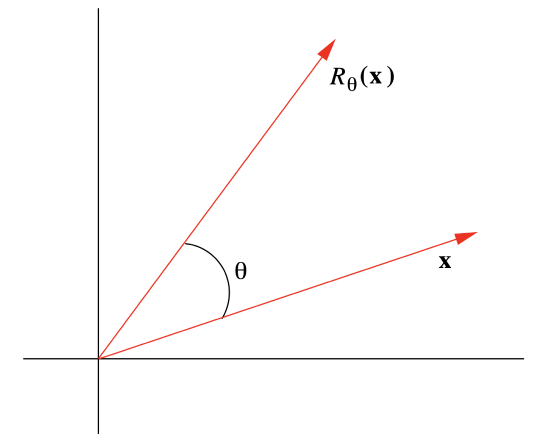
Example 1.5.6
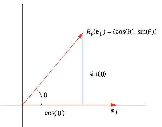
Let Rθ:R2→R2 be the function that rotates a vector x in R2 counterclockwise through an angle θ, as shown in Figure 1.5.1. Geometrically, it seems reasonable that Rθ is a linear function; that is, rotating the vector x+y through an angle θ should give the same result as first rotating x and y separately through an angle θ and then adding, and rotating a vector ax through an angle θ should give the same result as first rotating x through an angle θ and then multiplying by a. Now, from the definition of cos(θ) and sin(θ),
Rθ(e1)=Rθ(1,0)=(cos(θ),sin(θ))
(see Figure 1.5.2), and, since e2 is e1 rotated, counterclockwise, through an angle π2,
Rθ(e2)=Rθ+π2(e1)=(cos(θ+π2),sin(θ+π2))=(−sin(θ),cos(θ)).
Rθ(x,y)=[cos(θ)−sin(θ)sin(θ)cos(θ)][xy].
You are asked in Exercise 9 to verify that the linear function defined in (???) does in fact rotate vectors through an angle θ in the counterclockwise direction. Note that, for example, when θ=π2, we have
Rπ2(x,y)=[0−110][xy].
In particular, note that Rπ2(1,0)=(0,1) and Rπ2(0,1)=(−1,0); that is, Rπ2 takes e1 to e2 and e2 to −e1. For another example, if θ=π6, then
Rπ6(x,y)=[√32−1212√32][xy].
In particular,
Rπ6(1,2)=[√32−1212√32][12]=[√32−112+√3]=[√3−221+2√32].
Affine functions
Definition 1.5.2
We say a function A:Rm→Rn is affine if there is a linear function L:Rm→Rn and a vector b in Rn such that
A(x)=L(x)+b
for all x in Rm.
An affine function is just a linear function plus a translation. From our knowledge of linear functions, it follows that if A:Rm→Rn is affine, then there is an n×m matrix M and a vector b in Rn such that
A(x)=Mx+b
for all x in Rm. In particular, if f:R→R is affine, then there are real numbers m and b such that
f(x)=mx+b
for all real numbers x.
Example 1.5.7
The function
A(x,y)=(2x+3,y−4x+1)
is an affine function from R2 to R2 since we may write it in the form
A(x,y)=L(x,y)+(3,1),
where L is the linear function
L(x,y)=(2x,y−4x).
Note that L(1,0)=(2,−4) and L(0,1)=(0,1), so we may also write A in the form
A(x,y)=[20−41][xy]+[31].
Example 1.5.8
The affine function
A(x,y)=[1√2−1√21√21√2][xy]+[12]
first rotates a vector, counterclockwise, in R2 through an angle of π4 and then translates it by the vector (1,2).