8.6: Laplace’s Equation in 2D, Revisited
- Page ID
- 90969

\( \newcommand{\vecs}[1]{\overset { \scriptstyle \rightharpoonup} {\mathbf{#1}} } \)
\( \newcommand{\vecd}[1]{\overset{-\!-\!\rightharpoonup}{\vphantom{a}\smash {#1}}} \)
\( \newcommand{\id}{\mathrm{id}}\) \( \newcommand{\Span}{\mathrm{span}}\)
( \newcommand{\kernel}{\mathrm{null}\,}\) \( \newcommand{\range}{\mathrm{range}\,}\)
\( \newcommand{\RealPart}{\mathrm{Re}}\) \( \newcommand{\ImaginaryPart}{\mathrm{Im}}\)
\( \newcommand{\Argument}{\mathrm{Arg}}\) \( \newcommand{\norm}[1]{\| #1 \|}\)
\( \newcommand{\inner}[2]{\langle #1, #2 \rangle}\)
\( \newcommand{\Span}{\mathrm{span}}\)
\( \newcommand{\id}{\mathrm{id}}\)
\( \newcommand{\Span}{\mathrm{span}}\)
\( \newcommand{\kernel}{\mathrm{null}\,}\)
\( \newcommand{\range}{\mathrm{range}\,}\)
\( \newcommand{\RealPart}{\mathrm{Re}}\)
\( \newcommand{\ImaginaryPart}{\mathrm{Im}}\)
\( \newcommand{\Argument}{\mathrm{Arg}}\)
\( \newcommand{\norm}[1]{\| #1 \|}\)
\( \newcommand{\inner}[2]{\langle #1, #2 \rangle}\)
\( \newcommand{\Span}{\mathrm{span}}\) \( \newcommand{\AA}{\unicode[.8,0]{x212B}}\)
\( \newcommand{\vectorA}[1]{\vec{#1}} % arrow\)
\( \newcommand{\vectorAt}[1]{\vec{\text{#1}}} % arrow\)
\( \newcommand{\vectorB}[1]{\overset { \scriptstyle \rightharpoonup} {\mathbf{#1}} } \)
\( \newcommand{\vectorC}[1]{\textbf{#1}} \)
\( \newcommand{\vectorD}[1]{\overrightarrow{#1}} \)
\( \newcommand{\vectorDt}[1]{\overrightarrow{\text{#1}}} \)
\( \newcommand{\vectE}[1]{\overset{-\!-\!\rightharpoonup}{\vphantom{a}\smash{\mathbf {#1}}}} \)
\( \newcommand{\vecs}[1]{\overset { \scriptstyle \rightharpoonup} {\mathbf{#1}} } \)
\( \newcommand{\vecd}[1]{\overset{-\!-\!\rightharpoonup}{\vphantom{a}\smash {#1}}} \)
\(\newcommand{\avec}{\mathbf a}\) \(\newcommand{\bvec}{\mathbf b}\) \(\newcommand{\cvec}{\mathbf c}\) \(\newcommand{\dvec}{\mathbf d}\) \(\newcommand{\dtil}{\widetilde{\mathbf d}}\) \(\newcommand{\evec}{\mathbf e}\) \(\newcommand{\fvec}{\mathbf f}\) \(\newcommand{\nvec}{\mathbf n}\) \(\newcommand{\pvec}{\mathbf p}\) \(\newcommand{\qvec}{\mathbf q}\) \(\newcommand{\svec}{\mathbf s}\) \(\newcommand{\tvec}{\mathbf t}\) \(\newcommand{\uvec}{\mathbf u}\) \(\newcommand{\vvec}{\mathbf v}\) \(\newcommand{\wvec}{\mathbf w}\) \(\newcommand{\xvec}{\mathbf x}\) \(\newcommand{\yvec}{\mathbf y}\) \(\newcommand{\zvec}{\mathbf z}\) \(\newcommand{\rvec}{\mathbf r}\) \(\newcommand{\mvec}{\mathbf m}\) \(\newcommand{\zerovec}{\mathbf 0}\) \(\newcommand{\onevec}{\mathbf 1}\) \(\newcommand{\real}{\mathbb R}\) \(\newcommand{\twovec}[2]{\left[\begin{array}{r}#1 \\ #2 \end{array}\right]}\) \(\newcommand{\ctwovec}[2]{\left[\begin{array}{c}#1 \\ #2 \end{array}\right]}\) \(\newcommand{\threevec}[3]{\left[\begin{array}{r}#1 \\ #2 \\ #3 \end{array}\right]}\) \(\newcommand{\cthreevec}[3]{\left[\begin{array}{c}#1 \\ #2 \\ #3 \end{array}\right]}\) \(\newcommand{\fourvec}[4]{\left[\begin{array}{r}#1 \\ #2 \\ #3 \\ #4 \end{array}\right]}\) \(\newcommand{\cfourvec}[4]{\left[\begin{array}{c}#1 \\ #2 \\ #3 \\ #4 \end{array}\right]}\) \(\newcommand{\fivevec}[5]{\left[\begin{array}{r}#1 \\ #2 \\ #3 \\ #4 \\ #5 \\ \end{array}\right]}\) \(\newcommand{\cfivevec}[5]{\left[\begin{array}{c}#1 \\ #2 \\ #3 \\ #4 \\ #5 \\ \end{array}\right]}\) \(\newcommand{\mattwo}[4]{\left[\begin{array}{rr}#1 \amp #2 \\ #3 \amp #4 \\ \end{array}\right]}\) \(\newcommand{\laspan}[1]{\text{Span}\{#1\}}\) \(\newcommand{\bcal}{\cal B}\) \(\newcommand{\ccal}{\cal C}\) \(\newcommand{\scal}{\cal S}\) \(\newcommand{\wcal}{\cal W}\) \(\newcommand{\ecal}{\cal E}\) \(\newcommand{\coords}[2]{\left\{#1\right\}_{#2}}\) \(\newcommand{\gray}[1]{\color{gray}{#1}}\) \(\newcommand{\lgray}[1]{\color{lightgray}{#1}}\) \(\newcommand{\rank}{\operatorname{rank}}\) \(\newcommand{\row}{\text{Row}}\) \(\newcommand{\col}{\text{Col}}\) \(\renewcommand{\row}{\text{Row}}\) \(\newcommand{\nul}{\text{Nul}}\) \(\newcommand{\var}{\text{Var}}\) \(\newcommand{\corr}{\text{corr}}\) \(\newcommand{\len}[1]{\left|#1\right|}\) \(\newcommand{\bbar}{\overline{\bvec}}\) \(\newcommand{\bhat}{\widehat{\bvec}}\) \(\newcommand{\bperp}{\bvec^\perp}\) \(\newcommand{\xhat}{\widehat{\xvec}}\) \(\newcommand{\vhat}{\widehat{\vvec}}\) \(\newcommand{\uhat}{\widehat{\uvec}}\) \(\newcommand{\what}{\widehat{\wvec}}\) \(\newcommand{\Sighat}{\widehat{\Sigma}}\) \(\newcommand{\lt}{<}\) \(\newcommand{\gt}{>}\) \(\newcommand{\amp}{&}\) \(\definecolor{fillinmathshade}{gray}{0.9}\)Harmonic functions are solutions of Laplace’s equation. We have seen that the real and imaginary parts of a holomorphic function are harmonic. So, there must be a connection between complex functions and solutions of the two-dimensional Laplace equation. In this section we will describe how conformal mapping can be used to find solutions of Laplace’s equation in two dimensional regions.
In Section 2.5 we had first seen applications in two-dimensional steadystate heat flow (or, diffusion), electrostatics, and fluid flow. For example, letting \(\phi(\mathbf{r})\) be the electric potential, one has for a static charge distribution, \(\rho(\mathbf{r})\), that the electric field, \(\mathbf{E}=\nabla \phi\), satisfies
\[\nabla \cdot \mathbf{E}=\rho / \epsilon_{0} .\nonumber \]
In regions devoid of charge, these equations yield the Laplace equation, \(\nabla^{2} \phi=0\).
Similarly, we can derive Laplace’s equation for an incompressible, \(\nabla \cdot \mathbf{v}=\) 0 , irrotational,,\(\nabla \times \mathbf{v}=0\), fluid flow. From well-known vector identities, we know that \(\nabla \times \nabla \phi=0\) for a scalar function, \(\phi\). Therefore, we can introduce a velocity potential, \(\phi\), such that \(\mathbf{v}=\nabla \phi\). Thus, \(\nabla \cdot \mathbf{v}=0\) implies \(\nabla^{2} \phi=0\). So, the velocity potential satisfies Laplace’s equation.
Fluid flow is probably the simplest and most interesting application of complex variable techniques for solving Laplace’s equation. So, we will spend some time discussing how conformal mappings have been used to study two-dimensional ideal fluid flow, leading to the study of airfoil design.
Fluid Flow
The study of fluid flow and conformal mappings dates back to Euler, Riemann, and others.\(^{1}\) The method was further elaborated upon by physicists like Lord Rayleigh (1877) and applications to airfoil theory we presented in papers by Kutta (1902) and Joukowski (1906) on later to be improved upon by others.
The physics behind flight and the dynamics of wing theory relies on the ideas of drag and lift. Namely, as the the cross section of a wing, the airfoil, goes through the air, it will experience several forces. The air speed above and belong the wing will differ due to the distance the air has to travel across the top and bottom of the wing. According to Bernoulli’s Principle, steady fluid flow satisfies the conservation of energy in the form
\[P+\frac{1}{2} \rho U^{2}+\rho g h=\text { constant }\nonumber \]
at points on either side of the wing profile. Here \(P\) is the pressure, \(\rho\) is the air density, \(U\) is the fluid speed, \(h\) is a reference height, and \(g\) is the acceleration due to gravity. The gravitational potential energy, \(\rho g h\), is roughly constant on either side of the wing. So, this reduces to
\[P+\frac{1}{2} \rho U^{2}=\text { constant. }\nonumber \]
Therefore, if the speed of the air below the wing is lower that than above the wing, the pressure below the wing will be higher, resulting in a net upward pressure. Since the pressure is the force per area, this will result in an upward force, a lift force, acting on the wing. This is the simplified version for the lift force. There is also a drag force acting in the direction of the flow. In general, we want to use complex variable methods to model the streamlines of the airflow as the air flows around an airfoil.
We begin by considering the fluid flow across a curve, \(C\) as shown in Figure \(\PageIndex{1}\). We assume that it is an ideal fluid with zero viscosity (i.e., does not flow like molasses) and is incompressible. It is a continuous, homogeneous flow with a constant thickness and represented by a velocity \(\mathbf{U}=(u(x, y), v(x, y))\), where \(u\) and \(v\) are the horizontal components of the flow as shown in Figure \(\PageIndex{1}\).
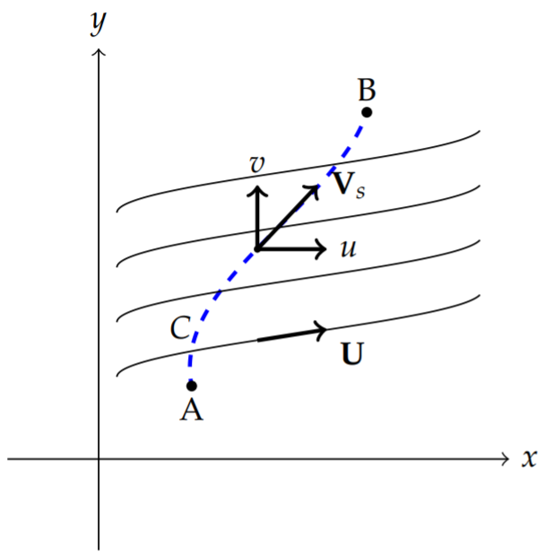
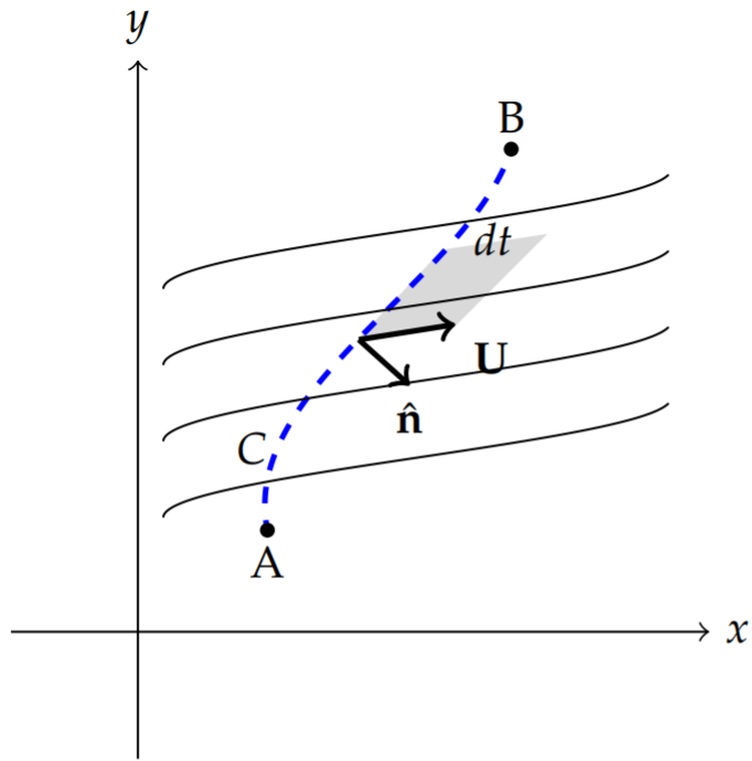
We are interested in the flow of fluid across a given curve which crosses several streamlines. The mass that flows over \(C\) per unit thickness in time \(d t\) can be given by
\[d m=\rho \mathbf{U} \cdot \hat{\mathbf{n}} d A d t .\nonumber \]
Here \(\hat{\mathbf{n}} d A\) is the normal area to the flow and for unit thickness can be written as \(\hat{\mathbf{n}} d A=\mathbf{i} d y-\mathbf{i} d x\). Therefore, for a unit thickness the mass flow rate is given by
\[\frac{d m}{d t}=\rho(u d y-v d x) .\nonumber \]
Since the total mass flowing across \(d s\) in time \(d t\) is given by \(d m=\rho d V\), for constant density, this also gives the volume flow rate,
\[\frac{d V}{d t}=u d y-v d x\nonumber \]
over a section of the curve. The total volume flow over \(C\) is therefore
\[\left.\frac{d V}{d t}\right|_{\text {total }}=\int_{C} u d y-v d x .\nonumber \]
If this flow is independent of the curve, i.e., the path, then we have
\[\frac{\partial u}{\partial x}=-\frac{\partial v}{\partial y} \text {. }\nonumber \]
[This is just a consequence of Green’s Theorem in the Plane. See Equation (8.1.3).] Another way to say this is that there exists a function, \(\psi(x, t)\), such that \(d \psi=u d y-v d x\). Then,
\[\int_{C} u d y-v d x=\int_{A}^{B} d \psi=\psi_{B}-\psi_{A} .\nonumber \]
However, from basic calculus of several variables, we know that
\[d \psi=\frac{\partial \psi}{\partial x} d x+\frac{\partial \psi}{\partial y} d y=u d y-v d x .\nonumber \]
Therefore,
\[u=\frac{\partial \psi}{\partial y}, \quad v=-\frac{\partial \psi}{\partial x} .\nonumber \]
It follows that if \(\psi(x, y)\) has continuous second derivatives, then \(u_{x}=-v_{y}\). This function is called the streamline function.
Furthermore, for constant density, we have
\[\begin{align} \nabla \cdot(\rho \mathbf{U}) &=\rho\left(\frac{\partial u}{\partial x}+\frac{\partial v}{\partial y}\right)\nonumber \\ &=\rho\left(\frac{\partial^{2} \psi}{\partial y \partial x} \frac{\partial^{2} \psi}{\partial x \partial y}\right)=0 .\label{eq:1} \end{align} \]
This is the conservation of mass formula for constant density fluid flow.
We can also assume that the flow is irrotational. This means that the vorticity of the flow vanishes; i.e., \(\nabla \times \mathbf{U}=0\). Since the curl of the velocity field is zero, we can assume that the velocity is the gradient of a scalar function, \(\mathbf{U}=\nabla \phi\). Then, a standard vector identity automatically gives
\[\nabla \times \mathbf{U}=\nabla \times \nabla \phi=0 .\nonumber \]
For the two-dimensional flow with \(\mathbf{U}=(u, v)\), we have
\[u=\frac{\partial \phi}{\partial x}, \quad v=\frac{\partial \phi}{\partial y} .\nonumber \]
This is the velocity potential function for the flow.
Let’s place the two-dimensional flow in the complex plane. Let an arbitrary point be \(z=(x, y)\). Then, we have found two real-valued functions, \(\psi(x, y)\) and \(\psi(x, y)\), satisfying the relations
\[\begin{align} &u=\frac{\partial \phi}{\partial x}=\frac{\partial \psi}{\partial y}\nonumber \\ &v=\frac{\partial \phi}{\partial y}=-\frac{\partial \psi}{\partial x}\label{eq:2} \end{align} \]
These are the Cauchy-Riemann relations for the real and imaginary parts of a complex differentiable function,
\[F(z(x, y)=\phi(x, y)+i \psi(x, y) .\nonumber \]
From its form, \(\frac{d F}{d z}\) is called the complex velocity and \(\sqrt{\left|\frac{d F}{d z}\right|}=\sqrt{u^{2}+v^{2}}\) is the flow speed.
Furthermore, we have
\[\frac{d F}{d z}= \frac{\partial \phi}{\partial x}+i \frac{\partial \psi}{\partial x}=u-i v .\nonumber \]
Integrating, we have
\[\begin{align} F=& \int_{C}(u-i v) d z\nonumber \\ \phi(x, y)+i \psi(x, y)=& \int_{\left(x_{0}, y_{0}\right)}^{(x, y)}[u(x, y) d x+v(x, y) d y]\nonumber \\ &+i \int_{\left(x_{0}, y_{0}\right)}^{(x, y)}[-v(x, y) d x+u(x, y) d y] .\label{eq:3} \end{align} \]
Therefore, the streamline and potential functions are given by the integral forms
\[\begin{align} &\phi(x, y)=\int_{\left(x_{0}, y_{0}\right)}^{(x, y)}[u(x, y) d x+v(x, y) d y],\nonumber \\ &\psi(x, y)=\int_{\left(x_{0}, y_{0}\right)}^{(x, y)}[-v(x, y) d x+u(x, y) d y] .\label{eq:4} \end{align} \]
These integrals give the circulation \(\int_{C} V_{s} d s=\int_{C} u d x+v d y\) and the fluid flow per time, \(\int_{C}-v d x+u d y\).
The streamlines for the flow are given by the level curves \(\psi(x, y)=c_{1}\) and the potential lines are given by the level curves \(\phi(x, y)=c_{2}\). These are two orthogonal families of curves; i.e., these families of curves intersect each other orthogonally at each point as we will see in the examples. Note that these families of curves also provide the field lines and equipotential curves for electrostatic problems.
Streamliners and potential curves are orthogonal families of curves.
Show that \(\phi(x, y)=c_{1}\) and \(\psi(x, y)=c_{2}\) are an orthogonal family of curves when \(F(z)=\phi(x, y)+i \psi(x, y)\) is holomorphic.
Solution
In order to show that these curves are orthogonal, we need to find the slopes of the curves at an arbitrary point, \((x, y)\). For \(\phi(x, y)=c_{1}\), we recall from multivaribale calculus that
\[d \phi=\frac{\partial \phi}{\partial x} d x+\frac{\partial \phi}{\partial y} d y=0 .\nonumber \]
So, the slope is found as
\[\frac{d y}{d x}=-\frac{\frac{\partial \phi}{\partial x}}{\frac{\partial \phi}{\partial y}}\nonumber \]
Similarly, we have
\[\frac{d y}{d x}=-\frac{\frac{\partial \psi}{\partial x}}{\frac{\partial \psi}{\partial y}} \text {. }\nonumber \]
Since \(F(z)\) is differentiable, we can use the Cauchy-Riemann equations to find the product of the slopes satisfy
\[\frac{\partial \phi}{\frac{\partial \phi}{\partial \phi} \frac{\partial \psi}{\partial x}}{\frac{\partial \psi}{\partial y}}=-\frac{\frac{\partial \psi}{\partial y}}{\frac{\partial \psi}{\partial y}} \frac{\partial \psi}{\partial x}=-1 .\nonumber \]
Therefore, \(\phi(x, y)=c_{1}\) and \(\psi(x, y)=c_{2}\) form an orthogonal family of curves.
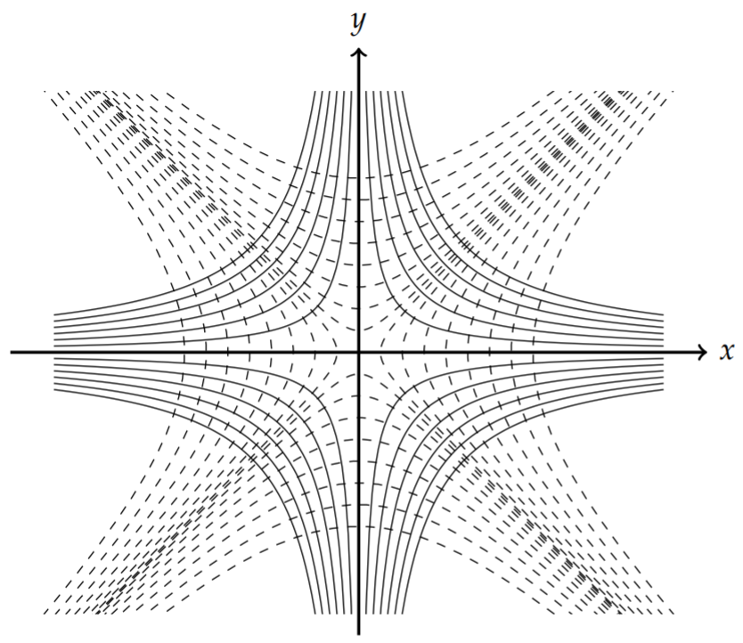
As an example, consider \(F(z)=z^{2}=x^{2}-y^{2}+2 i x y\). Then, \(\phi(x, y)=x^{2}-y^{2}\) and \(\psi(x, y)=2 x y\). The slopes of the families of curves are given by
\[\begin{align} \frac{d y}{d x} &=-\frac{\partial \phi}{\partial x}\nonumber \\ &=-\frac{2 x}{\partial y}=\frac{x}{y} .\nonumber \\ \frac{d y}{d x} &=-\frac{\frac{\partial \psi}{\partial x}}{\frac{\partial \psi}{\partial y}}\nonumber \\ &=-\frac{2 y}{2 x}=-\frac{y}{x} .\label{eq:5} \end{align} \]
The products of these slopes is \(-1\). The orthogonal families are depicted in Figure \(\PageIndex{3}\).
We will now turn to some typical examples by writing down some differentiable functions, \(F(z)\), and determining the types of flows that result from these examples. We will then turn in the next section to using these basic forms to solve problems in slightly different domains through the use of conformal mappings.
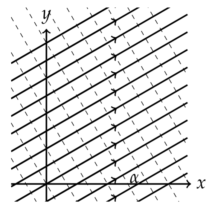
Describe the fluid flow associated with \(F(z)=U_{0} e^{-i \alpha} z\), where \(U_{0}\) and \(\alpha\) are real.
Solution
For this example, we have
\[\frac{dF}{dz}=U_0e^{-i\alpha}=u-iv.\nonumber \]
Thus, the velocity is constant,
\[\mathbf{U}=\left(U_{0} \cos \alpha, U_{0} \sin \alpha\right)\nonumber \]
Thus, the velocity is a uniform flow at an angle of \(\alpha\).
Since
\[F(z)=U_{0} e^{-i \alpha} z=U_{0}(x \cos \alpha+y \sin \alpha)+i U_{0}(y \cos \alpha-x \sin \alpha) .\nonumber \]
Thus, we have
\[\begin{align} &\phi(x, y)=U_{0}(x \cos \alpha+y \sin \alpha),\nonumber \\ &\psi(x, y)=U_{0}(y \cos \alpha-x \sin \alpha) .\label{eq:6} \end{align} \]
An example of this family of curves is shown in Figure \(\PageIndex{4}\).
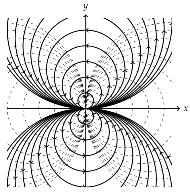
Describe the flow given by \(F(z)=\frac{u_{0} e^{-i \alpha}}{z-z_{0}}\).
Solution
We write
\[\begin{align} F(z)=& \frac{U_{0} e^{-i \alpha}}{z-z_{0}}\nonumber \\ =& \frac{U_{0}(\cos \alpha+i \sin \alpha)}{\left(x-x_{0}\right)^{2}+\left(y-y_{0}\right)^{2}}\left[\left(x-x_{0}\right)-i\left(y-y_{0}\right)\right]\nonumber \\ =& \frac{U_{0}}{\left(x-x_{0}\right)^{2}+\left(y-y_{0}\right)^{2}}\left[\left(x-x_{0}\right) \cos \alpha+\left(y-y_{0}\right) \sin \alpha\right]\nonumber \\ &+i \frac{U_{0}}{\left(x-x_{0}\right)^{2}+\left(y-y_{0}\right)^{2}}\left[-\left(y-y_{0}\right) \cos \alpha+\left(x-x_{0}\right) \sin \alpha\right] .\label{eq:7} \end{align} \]
The level curves become
\[\begin{align} &\phi(x, y)=\frac{U_{0}}{\left(x-x_{0}\right)^{2}+\left(y-y_{0}\right)^{2}}\left[\left(x-x_{0}\right) \cos \alpha+\left(y-y_{0}\right) \sin \alpha\right]=c_{1},\nonumber \\ &\psi(x, y)=\frac{U_{0}}{\left(x-x_{0}\right)^{2}+\left(y-y_{0}\right)^{2}}\left[-\left(y-y_{0}\right) \cos \alpha+\left(x-x_{0}\right) \sin \alpha\right]=c_{2} .\label{eq:8} \end{align} \]
The level curves for the stream and potential functions satisfy equations of the form
\[\beta_{i}\left(\Delta x^{2}+\Delta y^{2}\right)-\cos \left(\alpha+\delta_{i}\right) \Delta x-\sin \left(\alpha+\delta_{i}\right) \Delta y=0,\nonumber \]
where \(\Delta x=x-x_{0}, \Delta y=y-y_{0}, \beta_{i}=\frac{c_{i}}{U_{0}}, \delta_{1}=0\), and \(\delta_{2}=\pi / 2\)., These can be written in the more suggestive form
\[\left(\Delta x-\gamma_{i} \cos \left(\alpha-\delta_{i}\right)\right)^{2}+\left(\Delta y-\gamma_{i} \sin \left(\alpha-\delta_{i}\right)\right)^{2}=\gamma_{i}^{2}\nonumber \]
for \(\gamma_{i}=\frac{c_{i}}{2 U_{0}}, i=1,2\). Thus, the stream and potential curves are circles with varying radii \(\left(\gamma_{i}\right)\) and centers \(\left(\left(x_{0}+\gamma_{i} \cos \left(\alpha-\delta_{i}\right), y_{0}+\gamma_{i} \sin \left(\alpha-\delta_{i}\right)\right)\right.\) ). Examples of this family of curves is shown for \(\alpha=0\) in in Figure \(\PageIndex{5}\) and for \(\alpha=\pi / 6\) in in Figure \(\PageIndex{6}\).
The components of the velocity field for \(\alpha=0\) are found from
\[\begin{align} \frac{d F}{d z} &=\frac{d}{d z}\left(\frac{U_{0}}{z-z_{0}}\right)\nonumber \\ &=-\frac{U_{0}}{\left(z-z_{0}\right)^{2}}\nonumber \\ &=-\frac{U_{0}\left[\left(x-x_{0}\right)-i\left(y-y_{0}\right)\right]^{2}}{\left[\left(x-x_{0}\right)^{2}+\left(y-y_{0}\right)^{2}\right]^{2}}\nonumber \\ &=-\frac{U_{0}\left[\left(x-x_{0}\right)^{2}+\left(y-y_{0}\right)^{2}-2 i\left(x-x_{0}\right)\left(y-y_{0}\right)\right]}{\left[\left(x-x_{0}\right)^{2}+\left(y-y_{0}\right)^{2}\right]^{2}}\nonumber \\ &=-\frac{U_{0}\left[\left(x-x_{0}\right)^{2}+\left(y-y_{0}\right)^{2}\right]}{\left[\left(x-x_{0}\right)^{2}+\left(y-y_{0}\right)^{2}\right]^{2}}+i \frac{U_{0}\left[2\left(x-x_{0}\right)\left(y-y_{0}\right)\right]}{\left[\left(x-x_{0}\right)^{2}+\left(y-y_{0}\right)^{2}\right]^{2}}\nonumber \\ &=-\frac{U_{0}}{\left[\left(x-x_{0}\right)^{2}+\left(y-y_{0}\right)^{2}\right]}+i \frac{U_{0}\left[2\left(x-x_{0}\right)\left(y-y_{0}\right)\right]}{\left[\left(x-x_{0}\right)^{2}+\left(y-y_{0}\right)^{2}\right]^{2}} .\label{eq:9} \end{align} \]
Thus, we have
\[\begin{align} u &=-\frac{U_{0}}{\left[\left(x-x_{0}\right)^{2}+\left(y-y_{0}\right)^{2}\right]^{\prime}}\nonumber \\ v &=\frac{U_{0}\left[2\left(x-x_{0}\right)\left(y-y_{0}\right)\right]}{\left[\left(x-x_{0}\right)^{2}+\left(y-y_{0}\right)^{2}\right]^{2}} .\label{eq:10} \end{align} \]
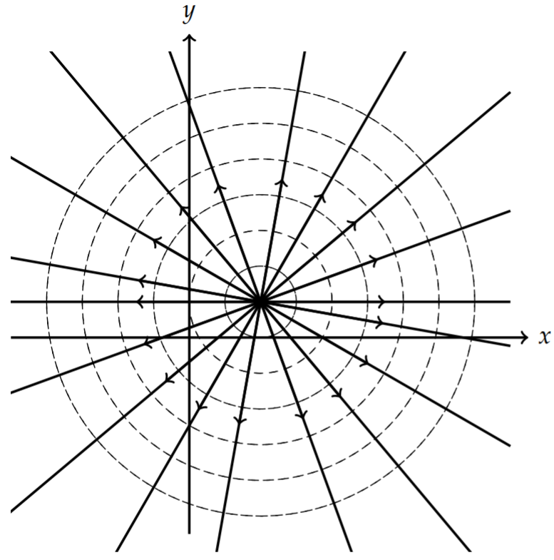
Describe the flow given by \(F(z)=\frac{m}{2 \pi} \ln \left(z-z_{0}\right)\).
Solution
We write \(F(z)\) in terms of its real and imaginary parts:
\[\begin{align} F(z) &=\frac{m}{2 \pi} \ln \left(z-z_{0}\right)\nonumber \\ &=\frac{m}{2 \pi}\left[\ln \sqrt{\left(x-x_{0}\right)^{2}+\left(y-y_{0}\right)^{2}}+i \tan ^{-1} \frac{y-y_{0}}{x-x_{0}}\right] .\label{eq:11} \end{align} \]
The level curves become
\[\begin{align} &\phi(x, y)=\frac{m}{2 \pi} \ln \sqrt{\left(x-x_{0}\right)^{2}+\left(y-y_{0}\right)^{2}}=c_{1},\nonumber \\ &\psi(x, y)=\frac{m}{2 \pi} \tan ^{-1} \frac{y-y_{0}}{x-x_{0}}=c_{2} .\label{eq:12} \end{align} \]
Rewriting these equations, we have
\[\begin{align} \left(x-x_{0}\right)^{2}+\left(y-y_{0}\right)^{2} &=e^{4 \pi c_{1} / m},\nonumber \\ y-y_{0} &=\left(x-x_{0}\right) \tan \frac{2 \pi c_{2}}{m} .\label{eq:13} \end{align} \]
In Figure \(\PageIndex{7}\) we see that the stream lines are those for a source or sink depending if \(m>0\) or \(m<0\), respectively.
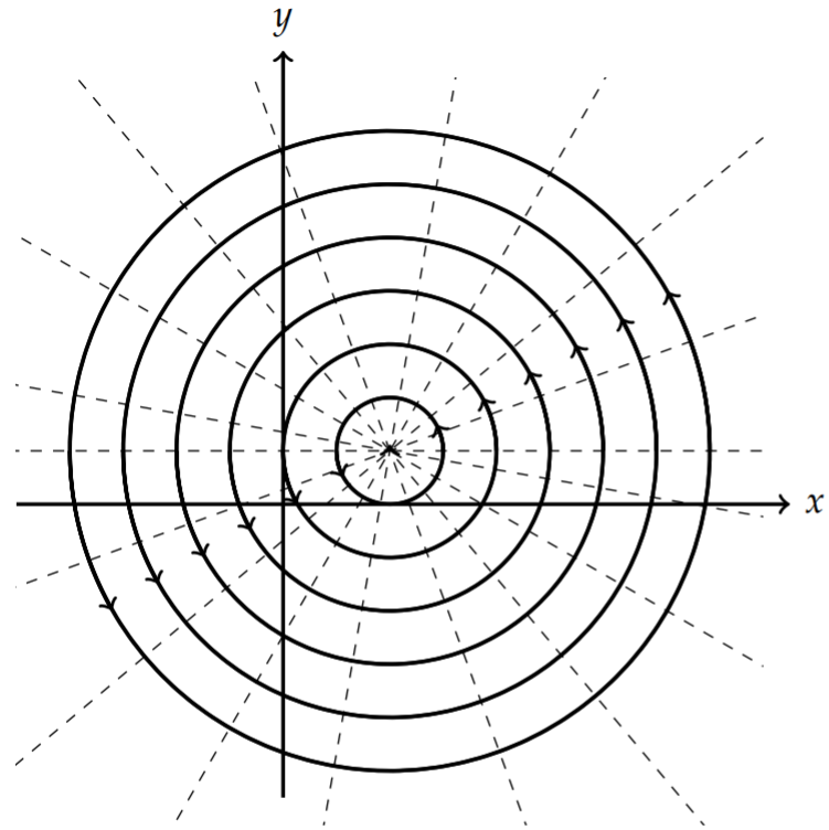
Describe the flow given by \(F(z)=-\frac{i \Gamma}{2 \pi} \ln \frac{z-z_{0}}{a}\).
Solution
We write \(F(z)\) in terms of its real and imaginary parts:
\[\begin{align} F(z) &=-\frac{i \Gamma}{2 \pi} \ln \frac{z-z_{0}}{a}\nonumber \\ &=-i \frac{\Gamma}{2 \pi} \ln \sqrt{\left(\frac{x-x_{0}}{a}\right)^{2}+\left(\frac{y-y_{0}}{a}\right)^{2}}+\frac{\Gamma}{2 \pi} \tan ^{-1} \frac{y-y_{0}}{x-x_{0}}\label{eq:14} \end{align} \]
The level curves become
\[\begin{align} &\phi(x, y)=\frac{\Gamma}{2 \pi} \tan ^{-1} \frac{y-y_{0}}{x-x_{0}}=c_{1},\nonumber \\ &\psi(x, y)=-\frac{\Gamma}{2 \pi} \ln \sqrt{\left(\frac{x-x_{0}}{a}\right)^{2}+\left(\frac{y-y_{0}}{a}\right)^{2}}=c_{2} .\label{eq:15} \end{align} \]
Rewriting these equations, we have
\[\begin{align} y-y_{0} &=\left(x-x_{0}\right) \tan \frac{2 \pi c_{1}}{\Gamma},\nonumber \\ \left(\frac{x-x_{0}}{a}\right)^{2}+\left(\frac{y-y_{0}}{a}\right)^{2} &=e^{-2 \pi c_{2} / \Gamma} .\label{eq:16} \end{align} \]
In Figure \(\PageIndex{8}\) we see that the stream lines circles, indicating rotational motion. Therefore, we have a vortex of counterclockwise, or clockwise flow, depending if \(\Gamma>0\) or \(\Gamma<0\), respectively.
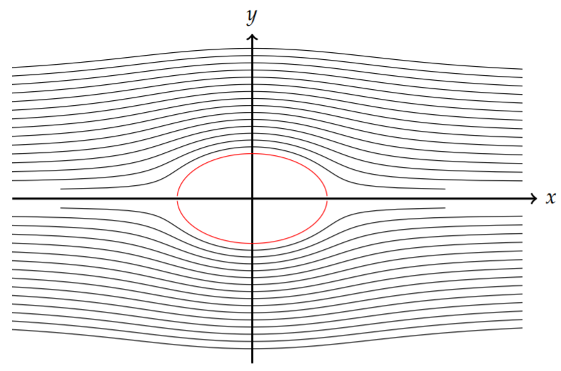
Flow around a cylinder, \(F(z)=U_{0}\left(z+\frac{a^{2}}{z}\right), a, U_{0} \in R\).
Solution
For this example, we have
\[\begin{align} F(z) &=U_{0}\left(z+\frac{a^{2}}{z}\right)\nonumber \\ &=U_{0}\left(x+i y+\frac{a^{2}}{x+i y}\right)\nonumber \\ &=U_{0}\left(x+i y+\frac{a^{2}}{x^{2}+y^{2}}(x-i y)\right)\nonumber \\ &=U_{0} x\left(1+\frac{a^{2}}{x^{2}+y^{2}}\right)+i U_{0} y\left(1-\frac{a^{2}}{x^{2}+y^{2}}\right) .\label{eq:17} \end{align} \]
The level curves become
\[\begin{align} &\phi(x, y)=U_{0} x\left(1+\frac{a^{2}}{x^{2}+y^{2}}\right)=c_{1},\nonumber \\ &\psi(x, y)=U_{0} y\left(1-\frac{a^{2}}{x^{2}+y^{2}}\right)=c_{2} .\label{eq:18} \end{align} \]
Note that for the streamlines when \(|z|\) is large, then \(\psi \sim V y\), or horizontal lines. For \(x^{2}+y^{2}=a^{2}\), we have \(\psi=0\). This behavior is shown in Figure \(\PageIndex{9}\) where we have graphed the solution for \(r \geq a\).
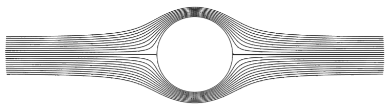
The level curves in Figure \(\PageIndex{9}\) can be obtained using the implicitplot feature of Maple. An example is shown below:
restart: with(plots):
k0:=20:
for k from 0 to k0 do
    P[k]:=implicitplot(sin(t)*(r-1/r)*1=(k0/2-k)/20, r=1..5,
    t=0..2*Pi, coords=polar,view=[-2..2, -1..1], axes=none,
    grid=[150,150],color=black):
    od:
display({seq(P[k],k=1..k0)},scaling=constrained);
A slight modification of the last example is if a circulation term is added:
\[F(z)=U_{0}\left(z+\frac{a^{2}}{z}\right)-\frac{i \Gamma}{2 \pi} \ln \frac{r}{a} .\nonumber \]
The combination of the two terms gives the streamlines,
\[\psi(x, y)=U_{0} y\left(1-\frac{a^{2}}{x^{2}+y^{2}}\right)-\frac{\Gamma}{2 \pi} \ln \frac{r}{a^{\prime}},\nonumber \]
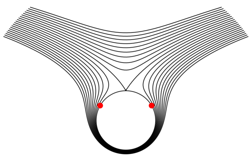
which are seen in Figure \(\PageIndex{10}\). We can see interesting features in this flow including what is called a stagnation point. A stagnation point is a point where the flow speed, \(\left|\frac{d F}{d z}\right|=0\).
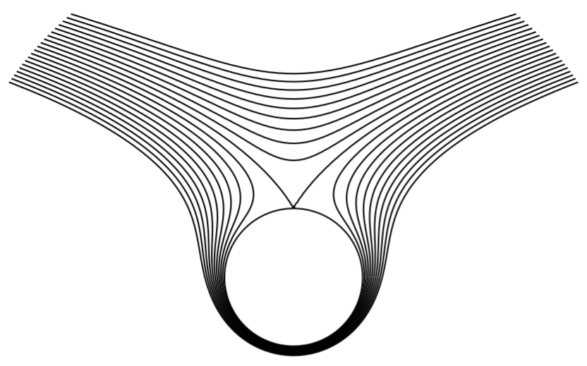
Find the stagnation point for the flow \(F(z)=\left(z+\frac{1}{z}\right)-i \ln z\).
Solution
Since the flow speed vanishes at the stagnation points, we consider
\[\frac{d F}{d z}=1-\frac{1}{z^{2}}-\frac{i}{z}=0 .\nonumber \]
This can be rewritten as
\[z^{2}-i z-1=0 \text {. }\nonumber \]
The solutions are \(z=\frac{1}{2}(i \pm \sqrt{3})\). Thus, there are two stagnation points on the cylinder about which the flow is circulating. These are shown in Figure \(\PageIndex{11}\).
Consider the complex potentials \(F(z)=\frac{k}{2 \pi} \ln \frac{z-a}{z-b}\), where \(k=q\) and \(k=-i\) for \(q\) real.
Solution
We first note that for \(z=x+i y\),
\[\begin{align} \ln \frac{z-a}{z-b}=& \ln \sqrt{(x-a)^{2}+y^{2}}-\ln \sqrt{(x-a)^{2}+y^{2}},\nonumber \\ &+i \tan ^{-1} \frac{y}{x-a}-i \tan ^{-1} \frac{y}{x-b} .\label{eq:19} \end{align} \]
For \(k=q\), we have
\[\begin{align} &\psi(x, y)=\frac{q}{2 \pi}\left[\ln \sqrt{(x-a)^{2}+y^{2}}-\ln \sqrt{(x-a)^{2}+y^{2}}\right]=c_{1},\nonumber \\ &\phi(x, y)=\frac{q}{2 \pi}\left[\tan ^{-1} \frac{y}{x-a}-\tan ^{-1} \frac{y}{x-b}\right]=c_{2} .\label{eq:20} \end{align} \]
The potential lines are circles and the streamlines are circular arcs as shown in Figure \(\PageIndex{12}\). These correspond to a source at \(z=a\) and a sink at \(z=b\). One can also view these as the electric field lines and equipotentials for an electric dipole consisting of two point charges of opposite sign at the points \(z=a\) and \(z=b\).
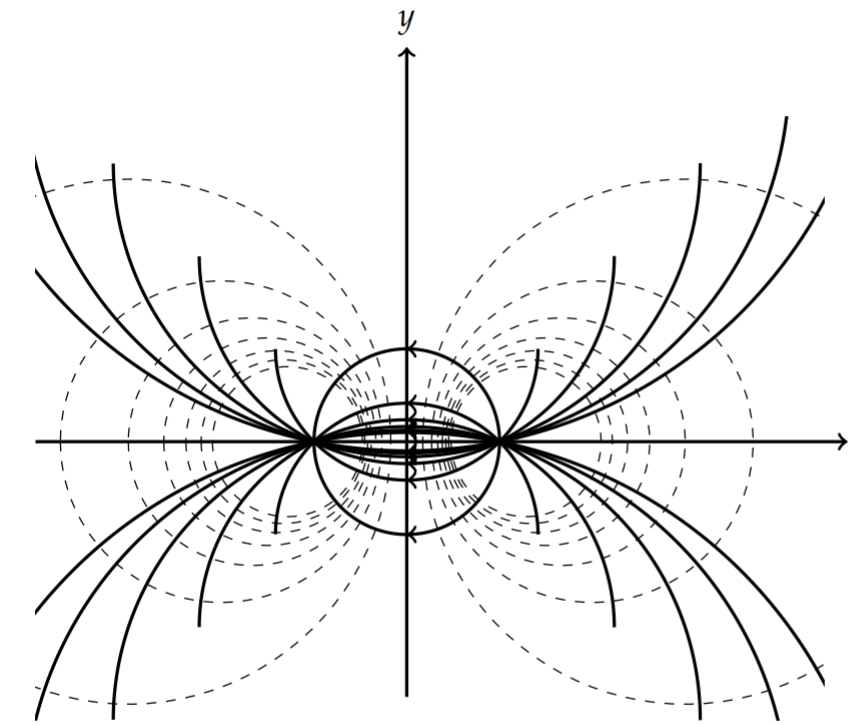
The equations for the curves are found from\(^{2}\)
\[\begin{align} (x-a)^{2}+y^{2} &=C_{1}\left[(x-b)^{2}+y^{2}\right],\nonumber \\ (x-a)(x-b)+y^{2} &=C_{2} y(a-b),\label{eq:21} \end{align} \]
where these can be rewritten, respectively, in the more suggestive forms
\[\begin{align} \left(x-\frac{a-b C_{1}}{1-C_{1}}\right)^{2}+y^{2} &=\frac{C_{1}(a-b)^{2}}{\left(1-C_{1}\right)^{2}}\nonumber \\ \left(x-\frac{a+b}{2}\right)^{2}+\left(y-\frac{C_{2}(a-b)}{2}\right)^{2} &=\left(1+C_{2}^{2}\right)\left(\frac{a-b}{2}\right)^{2}\label{eq:22} \end{align} \]
Note that the first family of curves are the potential curves and the second give the streamlines.
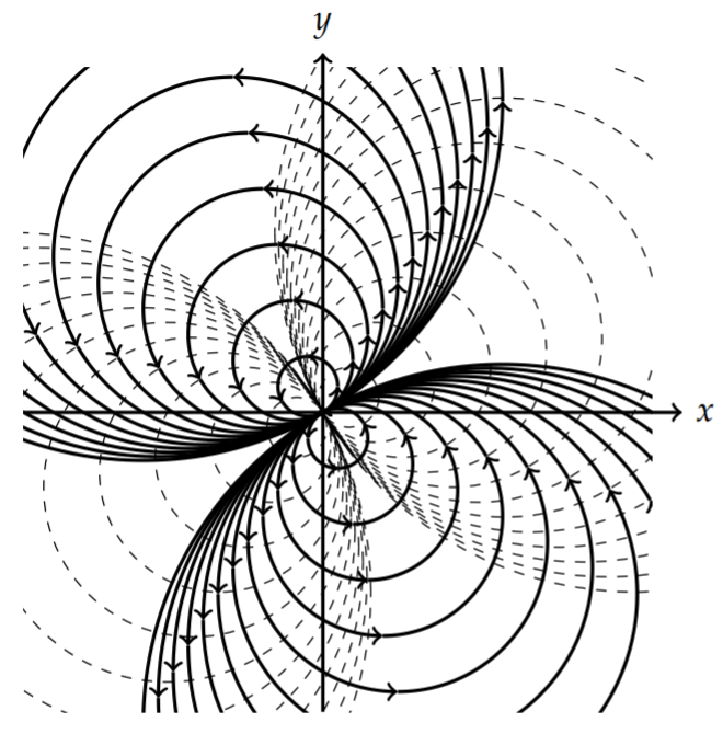
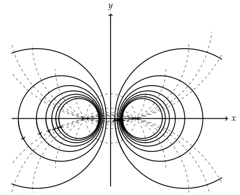
In the case that \(k=-i q\) we have
\[\begin{align} F(z)=& \frac{-i q}{2 \pi} \ln \frac{z-a}{z-b}\nonumber \\ =& \frac{-i q}{2 \pi}\left[\ln \sqrt{(x-a)^{2}+y^{2}}-\ln \sqrt{(x-a)^{2}+y^{2}}\right],\nonumber \\ &+\frac{q}{2 \pi}\left[\tan ^{-1} \frac{y}{x-a}-\tan ^{-1} \frac{y}{x-b}\right] .\label{eq:23} \end{align} \]
So, the roles of the streamlines and potential lines are reversed and the corresponding plots give a flow for a pair of vortices as shown in Figure \(\PageIndex{13}\).
Conformal Mappings
It would be nice if the complex potentials in the last section could be mapped to a region of the complex plane such that the new stream functions and velocity potentials represent new flows. In order for this to be true, we would need the new families to once again be orthogonal families of curves. Thus, the mappings we seek must preserve angles. Such mappings are called conformal mappings.
We let \(w=f(z)\) map points in the \(z\)-plane, \((x, y)\), to points in the \(w\) plane, \((u, v)\) by \(f(x+i y)=u+i v\). We have shown this in Figure 8.3.1.
Map lines in the \(z\)-plane to curves in the \(w\)-plane under \(f(z)=z^{2}\).
Solution
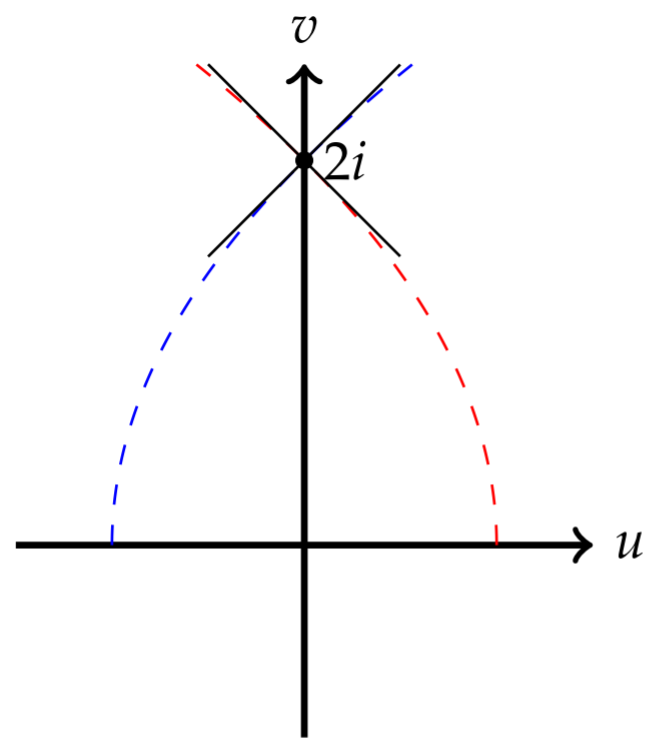
We have seen how grid lines in the \(z\)-plane is mapped by \(f(z)=z^{2}\) into the \(w\) plane in Figure 8.3.2, which is reproduced in Figure \(\PageIndex{14}\). The horizontal line \(x=1\) is mapped to \(u(1, y)=1-y^{2}\) and \(v(1, y)=2 y\). Eliminating the "parameter" \(y\) between these two equations, we have \(u=1-v^{2} / 4\). This is a parabolic curve. Similarly, the horizontal line \(y=1\) results in the curve \(u=v^{2} / 4-1\). These curves intersect at \(w=2 i\).
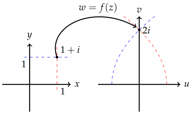
The lines in the z-plane intersect at \(z=1+i\) at right angles. In the w-plane we see that the curves \(u=1-v^{2} / 4\) and \(u=v^{2} / 4-1\) intersect at \(w=2 i\). The slopes of the tangent lines at \((0,2)\) are \(-1\) and 1 , respectively, as shown in Figure \(\PageIndex{15}\).
In general, if two curves in the \(z\)-plane intersect orthogonally at \(z=z_{0}\) and the corresponding curves in the \(w\)-plane under the mapping \(w=f(z)\) are orthogonal at \(w_{0}=f\left(z_{0}\right)\), then the mapping is conformal. As we have seen, holomorphic functions are conformal, but only at points where \(f^{\prime}(z) \neq\) \(0 .\)
Holomorphic functions are conformal at points where \(f^{\prime}(z) \neq 0\).
Images of the real and imaginary axes under \(f(z)=z^{2}\).
Solution
The line \(z=\) iy maps to \(w=z^{2}=-y^{2}\) and the line \(z=x\) maps to \(w=z^{2}=\) \(x^{2}\). The point of intersection \(z_{0}=0\) maps to \(w_{0}=0\). However, the image lines are the same line, the real axis in the w-plane. Obviously, the image lines are not orthogonal at the origin. Note that \(f^{\prime}(0)=0\).
One special mapping is the inversion mapping, which is given by
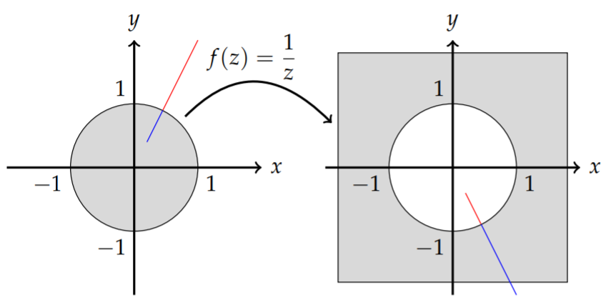
\[f(z)=\frac{1}{z} \text {. }\nonumber \]
This mapping maps the interior of the unit circle to the exterior of the unit circle in the \(w\)-plane as shown in Figure \(\PageIndex{16}\).
Let \(z=x+i y\), where \(x^{2}+y^{2}<1\). Then,
\[w=\frac{1}{x+i y}=\frac{x}{x^{2}+y^{2}}-i \frac{y}{x^{2}+y^{2}} .\nonumber \]
Thus, \(u=\frac{x}{x^{2}+y^{2}}\) and \(v=-\frac{y}{x^{2}+y^{2}}\), and
\[\begin{align} u^{2}+v^{2} &=\left(\frac{x}{x^{2}+y^{2}}\right)^{2}+\left(-\frac{y}{x^{2}+y^{2}}\right)^{2}\nonumber \\ &=\frac{x^{2}+y^{2}}{\left(x^{2}+y^{2}\right)^{2}}=\frac{1}{x^{2}+y^{2}}\label{eq:24} \end{align} \]
Thus, for \(x^{2}+y^{2}<1, u^{2}+U^{2}>1\). Furthermore, for \(x^{2}+y^{2}>1, u^{2}+U^{2}<\) 1 , and for \(x^{2}+y^{2}=1, u^{2}+U^{2}=1\).
In fact, an inversion maps circles into circles. Namely, for \(z=z_{0}+r e^{i \theta}\), we have
\[\begin{align} w &=\frac{1}{z_{0}+r e^{i \theta}}\nonumber \\ &=\frac{\bar{z}_{0}+r e^{-i \theta}}{\left|z_{0}+r e^{i \theta}\right|^{2}}\nonumber \\ &=w_{0}+R e^{-i \theta}\label{eq:25} \end{align} \]
Also, lines through the origin in the \(z\)-plane map into lines through the origin in the \(w\)-plane. Let \(z=x+i m x\). This corresponds to a line with slope \(m\) in the \(z\)-plane, \(y=m x\). It maps to
\[\begin{align} f(z) &=\frac{1}{z}\nonumber \\ &=\frac{1}{x+i m x}\nonumber \\ &=\frac{x-i m x}{\left(1+m^{2}\right) x} .\label{eq:26} \end{align} \]
So, \(u=\frac{x}{\left(1+m^{2}\right) x}\) and \(v=-\frac{m x}{\left(1+m^{2}\right) x}=-m u\). This is a line through the origin in the \(w\)-plane with slope \(-m\). This is shown in Figure \(\PageIndex{16}\). Note how the potion of the line \(y=2 x\) that is inside the unit disk maps to the outside of the disk in the \(w\)-plane.
The bilinear transformation.
Another interesting class of transformation, of which the inversion is contained, is the bilinear transformation. The bilinear transformation is given by
\[w=f(z)=\frac{a z+b}{c z+d}, \quad a d-b c \neq 0,\nonumber \]
where \(a, b, c\), and \(d\) are complex constants. These transformations were studied by mappings was studied by August Ferdinand Möbius (1790-1868) and are also called Möbius transformations, or linear fractional transformations. We further note that if \(a d-b c=0\), then the transformation reduces to the constat function.
We can seek to invert the transformation. Namely, solving for \(z\), we have
\[z=f^{-1}(w)=\frac{-d w+b}{c w-a}, \quad w \neq \frac{a}{c} .\nonumber \]
Since \(f^{-1}(w)\) is not defined for \(w \neq \frac{a}{c}\), we can say that \(w \neq \frac{a}{c}\) maps to the point at infinity, or \(f^{-1}\left(\frac{a}{c}\right)=\infty\). Similarly, we can let \(z \rightarrow \infty\) to obtain
\[f(\infty)=\lim _{n \rightarrow \infty} f(z)=-\frac{d}{c} .\nonumber \]
Thus, we have that the bilinear transformation is a one-to-one mapping of the extended complex \(z\)-plane to the extended complex \(w\)-plane.
The extended complex plane is the union of the complex plane plus the point at infinity. This is usually described in more detail using stereographic projection, which we will not review here.
If \(c=0, f(z)\) is easily seen to be a linear transformation. Linear transformations transform lines into lines and circles into circles.
When \(c \neq 0\), we can write
\[\begin{align} f(z) &=\frac{a z+b}{c z+d}\nonumber \\ &=\frac{c(a z+b)}{c(c z+d)}\nonumber \\ &=\frac{a c z+a d-a d+b c}{c(c z+d)}\nonumber \\ &=\frac{a(c z+d)-a d+b c}{c(c z+d)}\nonumber \\ &=\frac{a}{c}+\frac{b c-a d}{c} \frac{1}{c z+d} .\label{eq:27} \end{align} \]
We note that if \(b c-a d=0\), then \(f(z)=\frac{a}{c}\) is a constant, as noted above. The new form for \(f(z)\) shows that it is the composition of a linear function \(\zeta=\) \(c z+d\), an inversion, \(g(\zeta)=\frac{1}{\zeta}\), and another linear transformation, \(h(\zeta)=\) \(\frac{a}{c}+\frac{b c-a d}{c} \zeta\). Since linear transformations and inversions transform the set of circles and lines in the extended complex plane into circles and lines in the extended complex plane, then a bilinear does so as well.
What is important in out applications of complex analysis to the solution of Laplace’s equation in the transformation of regions of the complex plane into other regions of the complex plane. Needed transformations can be found using the following property of bilinear transformations:
A given set of three points in the \(z\)-plane can be transformed into a given set of points in the \(w\)-plane using a bilinear transformation.
This statement is based on the following observation: There are three independent numbers that determine a bilinear transformation. If \(a \neq 0\), then
\[\begin{align} f(z) &=\frac{a z+b}{c z+d}\nonumber \\ &=\frac{z+\frac{b}{a}}{\frac{c}{a} z+\frac{d}{a}}\nonumber \\ & \equiv \frac{z+\alpha}{\beta z+\gamma}\label{eq:28} \end{align} \]
For \(w=\frac{z+\alpha}{\beta z+\gamma}\), we have
\[\begin{align} w &=\frac{z+\alpha}{\beta z+\gamma}\nonumber \\ w(\beta z+\gamma) &=z+\alpha \nonumber \\ -\alpha+w z \beta+w \gamma &=z .\label{eq:29} \end{align} \]
Now, let \(w_{i}=f\left(z_{i}\right), i=1,2,3\). This gives three equations for the three unknowns \(\alpha, \beta\), and \(\gamma\). Namely,
\[\begin{align} &-\alpha+w_{1} z_{1} \beta+w_{1} \gamma=z_{1},\nonumber \\ &-\alpha+w_{2} z_{2} \beta+w_{2} \gamma=z_{2},\nonumber \\ &-\alpha+w_{3} z_{3} \beta+w_{3} \gamma=z_{3} .\label{eq:30} \end{align} \]
This systems of linear equation can be put into matrix form as
\[\left(\begin{array}{ccc} -1 & w_{1} z_{1} & w_{1} \\ -1 & w_{2} z_{2} & w_{2} \\ -1 & w_{3} z_{3} & w_{3} \end{array}\right)\left(\begin{array}{l} \alpha \\ \beta \\ \gamma \end{array}\right)=\left(\begin{array}{l} z_{1} \\ z_{2} \\ z_{3} \end{array}\right) \text {. }\nonumber \]
It is only a matter of solving this system for \((\alpha, \beta, \gamma)^{T}\) in order to find the bilinear transformation.
A quicker method is to use the implicit form of the transformation,
\[\frac{\left(z-z_{1}\right)\left(z_{2}-z_{3}\right)}{\left(z-z_{3}\right)\left(z_{2}-z_{1}\right)}=\frac{\left(w-w_{1}\right)\left(w_{2}-w_{3}\right)}{\left(w-w_{3}\right)\left(w_{2}-w_{1}\right)} .\nonumber \]
Note that this implicit relation works upon insertion of the values \(w_{i}, z_{i}\), for \(i=1,2,3\).
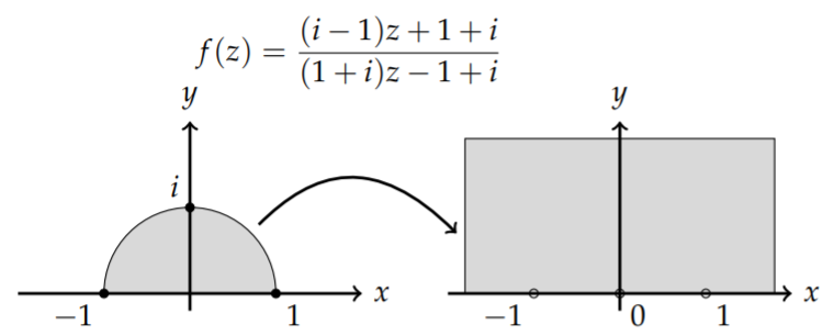
Find the bilinear transformation that maps the points \(-1, i, 1\) to the points \(-1,0,1\).
Solution
The implicit form of the transformation becomes
\[\begin{align} \frac{(z+1)(i-1)}{(z-1)(i+1)} &=\frac{(w+1)(0-1)}{(w-1)(0+1)}\nonumber \\ \frac{z+1}{z-1} \frac{i-1}{i+1} &=-\frac{w+1}{w-1}\label{eq:31} \end{align} \]
Solving for \(w\), we have
\[w=f(z)=\frac{(i-1) z+1+i}{(1+i) z-1+i} .\nonumber \]
We can use the transformation in the last example to map the unit disk containing the points \(-1, i\), and 1 to the half plane \(w>0\). We see that the unit circle gets mapped to the real axis with \(z=-i\) mapped to the point at infinity. The point \(z=0\) gets mapped to
\[w=\frac{1+i}{-1+i}=\frac{1+i}{-1+i} \frac{-1-i}{-1-i}=\frac{2}{2}=1 .\nonumber \]
Thus, interior points of the unit disk get mapped to the upper half plane. This is shown in Figure \(\PageIndex{17}\).