1: Mathematical Models of Biological Processes

Last updated
Save as PDF

Page ID: 36837

$ \newcommand{\vecs}[1]{\overset { \scriptstyle \rightharpoonup} {\mathbf{#1}} } $ $ \newcommand{\vecd}[1]{\overset{-\!-\!\rightharpoonup}{\vphantom{a}\smash {#1}}} $$\newcommand{\id}{\mathrm{id}}$ $ \newcommand{\Span}{\mathrm{span}}$ $ \newcommand{\kernel}{\mathrm{null}\,}$ $ \newcommand{\range}{\mathrm{range}\,}$ $ \newcommand{\RealPart}{\mathrm{Re}}$ $ \newcommand{\ImaginaryPart}{\mathrm{Im}}$ $ \newcommand{\Argument}{\mathrm{Arg}}$ $ \newcommand{\norm}[1]{\| #1 \|}$ $ \newcommand{\inner}[2]{\langle #1, #2 \rangle}$ $ \newcommand{\Span}{\mathrm{span}}$ $\newcommand{\id}{\mathrm{id}}$ $ \newcommand{\Span}{\mathrm{span}}$ $ \newcommand{\kernel}{\mathrm{null}\,}$ $ \newcommand{\range}{\mathrm{range}\,}$ $ \newcommand{\RealPart}{\mathrm{Re}}$ $ \newcommand{\ImaginaryPart}{\mathrm{Im}}$ $ \newcommand{\Argument}{\mathrm{Arg}}$ $ \newcommand{\norm}[1]{\| #1 \|}$ $ \newcommand{\inner}[2]{\langle #1, #2 \rangle}$ $ \newcommand{\Span}{\mathrm{span}}$$\newcommand{\AA}{\unicode[.8,0]{x212B}}$

Where are we going?

Science involves observations, formulation of hypotheses, and testing of hypotheses. This book is directed to quantifiable observations about living systems and hypotheses about the processes of life that are formulated as mathematical models. Using three biologically important examples, growth of the bacterium Vibrio natriegens, depletion of light below the surface of a lake or ocean, and growth of a mold colony, we demonstrate how to formulate mathematical models that lead to dynamic equations descriptive of natural processes. You will see how to compute solution equations to the dynamic equations and to test them against experimental data.

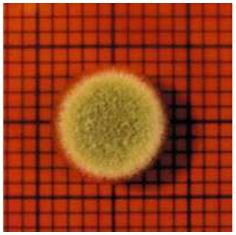
Examine the picture of the mold colony (Day 6 of Figure 1.14) and answer the question, “Where is the growth?” You will find the answer to be a fundamental component of the process.

$moldball.JPG$

In our language, a mathematical model is a concise verbal description of the interactions and forces that cause change with time or position of a biological system (or physical or economic or other system). The modeling process begins with a clear verbal statement based on the scientist’s understanding of the interactions and forces that govern change in the system. In order for mathematical techniques to assist in understanding the system, the verbal statement must be translated into an equation, called the dynamic equation of the model. Knowledge of the initial state of a system and the dynamic equation that describes the forces of change in the system is often sufficient to forecast an observed pattern of the system. A solution equation may be derived from the dynamic equation and an initial state of the system and a graph or table of values of the solution equation may then be compared with the observed pattern of nature. The extent to which solution equation matches the pattern is a measure of the validity of the mathematical model.

Mathematical modeling is used to describe the underlying mechanisms of a large number of processes in the natural or physical or social sciences. The chart in Figure 1.1 outlines the steps followed in finding a mathematical model.

Initially a scientist examines the biology of a problem, formulates a concise description, writes equations capturing the essence of the description, solves the equations, and makes predictions about the biological process. This path is marked by the bold arrows in Figure 1.1. It is seldom so simple! Almost always experimental data stimulates exchanges back and forth between a biologist and a computational scientist (mathematician, statistician, computer scientist) before a model is obtained that explains some of the biology. This additional exchange is represented by lightly marked arrows in Figure 1.1.

$biomath.JPG$

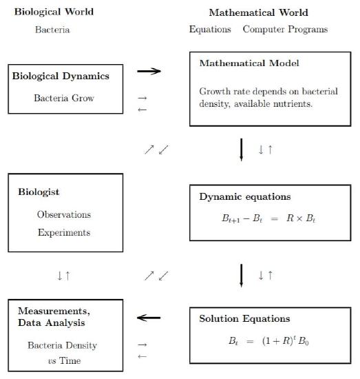
Figure $\PageIndex{1}$: Biology - Mathematics: Information flow chart for bacteria growth.

An initial approach to modeling may follow the bold arrows in Figure 1.1. For V. natriegens growth the steps might be:

The scientist ‘knows’ that 25% of the bacteria divide every 20 minutes.
If so, then bacteria increase, $B_{t+1} − B_t $, should be $0.25 B_t$ where $t$ marks time in 20-minute intervals and $B_t$ is the amount of bacteria at the end of the $t^{th}$ 20-minute interval.
From $B_{t+1} − B_{t} = 0.25 B_t $, the scientist may conclude that \[B_{t}=1.25^{t} B_{0}\] (More about this conclusion later).
The scientist uses this last equation to predict what bacteria density will be during an experiment in which V. natriegens, initially at $10^6$ cells per milliliter, are grown in a flask for two hours.
In the final stage, an experiment is carried out to grow the bacteria, their density is measured at selected times, and a comparison is made between observed densities and those predicted by equations. Reality usually strikes at this stage, for the observed densities may not match the predicted densities. If so, the additional network of lightly marked arrows of the chart is implemented.
Adjustments to a model of V. natriegen growth that may be needed include:
1. Different growth rate: A simple adjustment may be that only, say 20%, of the bacteria are dividing every 20 minutes and $B_{t} = 1.2^{t} B_0 $ matches experimental observations.
2. Variable growth rate: A more complex adjustment may be that initially 25% of the bacteria were dividing every 20 minutes but as the bacteria became more dense the growth rate fell to, say only 10% dividing during the last 20 minutes of the experiment.
3. Age dependent growth rate: A different adjustment may be required if initially all of the bacteria were from newly divided cells so that, for example, most of them grow without division during the first two 20-minute periods, and then divide during the third 20-minute interval.
4. Synchronous growth: A relatively easy adjustment may account for the fact that bacterial cell division is sometimes regulated by the photo period, causing all the bacteria to divide at a certain time of day. The green alga Chlamydomonas moewussi, for example, when grown in a laboratory with alternate 12 hour intervals of light and dark, accumulate nuclear subdivisions and each cell divides into eight cells at dawn of each day¹.

¹Emil Bernstein, Science 131 (1960), 1528.