1.1: Systems of Linear Equations
( \newcommand{\kernel}{\mathrm{null}\,}\)
- Understand the definition of Rn, and what it means to use Rn to label points on a geometric object.
- Pictures: solutions of systems of linear equations, parameterized solution sets.
- Vocabulary words: consistent, inconsistent, solution set.
During the first half of this textbook, we will be primarily concerned with understanding the solutions of systems of linear equations.
An equation in the unknowns x,y,z,… is called linear if both sides of the equation are a sum of (constant) multiples of x,y,z,…, plus an optional constant.
For instance,
3x+4y=2z−x−z=100
are linear equations, but
3x+yz=3sin(x)−cos(y)=2
are not.
We will usually move the unknowns to the left side of the equation, and move the constants to the right.
A system of linear equations is a collection of several linear equations, like
{x+2y+3z=62x−3y+2z=143x+y−z=−2.
- A solution of a system of equations is a list of numbers x,y,z,… that make all of the equations true simultaneously.
- The solution set of a system of equations is the collection of all solutions.
- Solving the system means finding all solutions with formulas involving some number of parameters.
A system of linear equations need not have a solution. For example, there do not exist numbers x and y making the following two equations true simultaneously:
{x+2y=3x+2y=−3.
In this case, the solution set is empty. As this is a rather important property of a system of equations, it has its own name.
A system of equations is called inconsistent if it has no solutions. It is called consistent otherwise.
A solution of a system of equations in n variables is a list of n numbers. For example, (x,y,z)=(1,−2,3) is a solution of (???). As we will be studying solutions of systems of equations throughout this text, now is a good time to fix our notions regarding lists of numbers.
Line, Plane, Space, Etc.
We use R to denote the set of all real numbers, i.e., the number line. This contains numbers like 0,32,−π,104,…
Let n be a positive whole number. We define
Rn=all ordered n-tuples of real numbers (x1,x2,x3,…,xn).
An n-tuple of real numbers is called a point of Rn.
In other words, Rn is just the set of all (ordered) lists of n real numbers. We will draw pictures of Rn in a moment, but keep in mind that this is the definition. For example, (0,32,−π) and (1,−2,3) are points of R3.
When n=1, we just get R back: R1=R. Geometrically, this is the number line.

Figure 1.1.1
When n=2, we can think of R2 as the xy-plane. We can do so because every point on the plane can be represented by an ordered pair of real numbers, namely, its x- and y-coordinates.
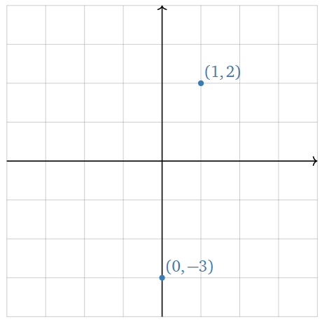
Figure 1.1.2
When n=3, we can think of R3 as the space we (appear to) live in. We can do so because every point in space can be represented by an ordered triple of real numebrs, namely, its x-, y-, and z-coordinates.
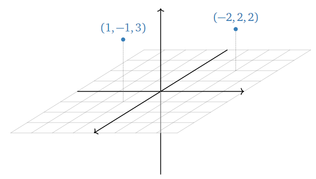
Figure 1.1.3
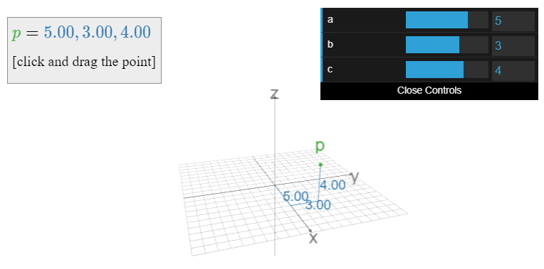
Figure 1.1.4: A point in 3-space, and its coordinates. Click and drag the point, or move the sliders.
So what is R4? or R5? or Rn? These are harder to visualize, so you have to go back to the definition: Rn is the set of all ordered n-tuples of real numbers (x1,x2,x3,…,xn).
They are still “geometric” spaces, in the sense that our intuition for R2 and R3 often extends to Rn.
We will make definitions and state theorems that apply to any Rn, but we will only draw pictures for R2 and R3.
The power of using these spaces is the ability to label various objects of interest, such as geometric objects and solutions of systems of equations, by the points of Rn.
All colors you can see can be described by three quantities: the amount of red, green, and blue light in that color. (Humans are trichromatic.) Therefore, we can use the points of R3 to label all colors: for instance, the point (.2,.4,.9) labels the color with 20% red, 40% green, and 90% blue intensity.
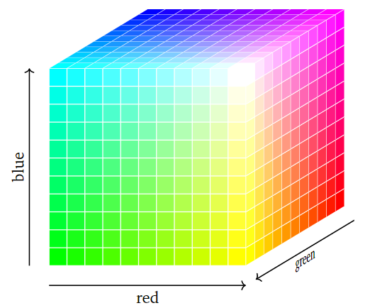
Figure 1.1.5
In the Overview, we could have used R4 to label the amount of traffic (x,y,z,w) passing through four streets. In other words, if there are 10,5,3,11 cars per hour passing through roads x,y,z,w, respectively, then this can be recorded by the point (10,5,3,11) in R4. This is useful from a psychological standpoint: instead of having four numbers, we are now dealing with just one piece of data.
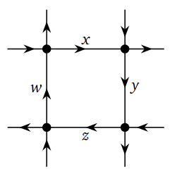
Figure 1.1.6
A QR code is a method of storing data in a grid of black and white squares in a way that computers can easily read. A typical QR code is a 29×29 grid. Reading each line left-to-right and reading the lines top-to-bottom (like you read a book) we can think of such a QR code as a sequence of 29×29=841 digits, each digit being 1 (for white) or 0 (for black). In such a way, the entire QR code can be regarded as a point in R841. As in the previous Example 1.1.6, it is very useful from a psychological perspective to view a QR code as a single piece of data in this way.


In the above examples, it was useful from a psychological perspective to replace a list of four numbers (representing traffic flow) or of 841 numbers (representing a QR code) by a single piece of data: a point in some Rn. This is a powerful concept; starting in Section 2.2, we will almost exclusively record solutions of systems of linear equations in this way.
Pictures of Solution Sets
Before discussing how to solve a system of linear equations below, it is helpful to see some pictures of what these solution sets look like geometrically.
Consider the linear equation x+y=1. We can rewrite this as y=1−x, which defines a line in the plane: the slope is −1, and the x-intercept is 1.
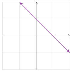
Figure 1.1.8
For our purposes, a line is a ray that is straight and infinite in both directions.
Consider the linear equation x+y+z=1. This is the implicit equation for a plane in space.
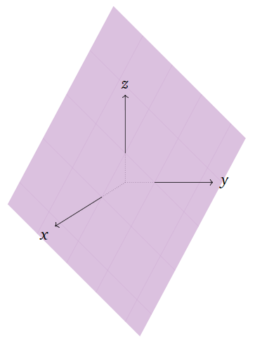
Figure 1.1.9
A plane is a flat sheet that is infinite in all directions.
The equation x+y+z+w=1 defines a “3-plane” in 4-space, and more generally, a single linear equation in n variables defines an “(n−1)-plane” in n-space. We will make these statements precise in Section 2.7.
Now consider the system of two linear equations
{x−3y=−3.2x+y=8.
Each equation individually defines a line in the plane, pictured below.
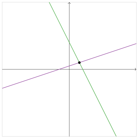
Figure 1.1.10
A solution to the system of both equations is a pair of numbers (x,y) that makes both equations true at once. In other words, it as a point that lies on both lines simultaneously. We can see in the picture above that there is only one point where the lines intersect: therefore, this system has exactly one solution. (This solution is (3,2), as the reader can verify.)
Usually, two lines in the plane will intersect in one point, but of course this is not always the case. Consider now the system of equations
{x−3y=−3.x−3y=3.
These define parallel lines in the plane.
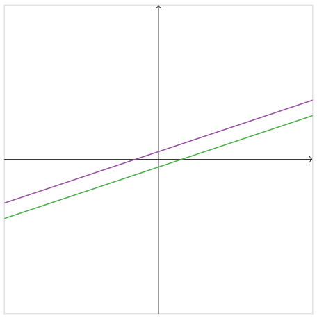
Figure 1.1.11
The fact that that the lines do not intersect means that the system of equations has no solution. Of course, this is easy to see algebraically: if x−3y=−3, then it is cannot also be the case that x−3y=3.
There is one more possibility. Consider the system of equations
{x−3y=−3.2x−6y=−6.
The second equation is a multiple of the first, so these equations define the same line in the plane.
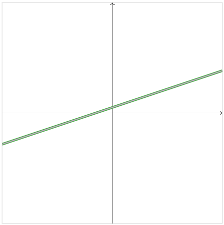
Figure 1.1.12
In this case, there are infinitely many solutions of the system of equations.
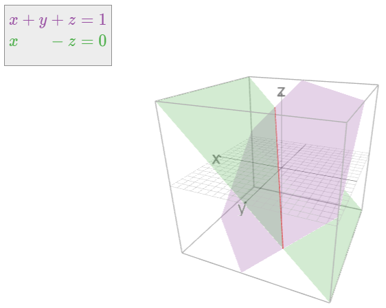
Consider the system of two linear equations
{x+y+z=1x−z=0.
Each equation individually defines a plane in space. The solutions of the system of both equations are the points that lie on both planes. We can see in the picture below that the planes intersect in a line. In particular, this system has infinitely many solutions.
In general, the solutions of a system of equations in n variables is the intersection of “(n−1)-planes” in n-space. This is always some kind of linear space, as we will discuss in Section 2.4.
Parametric Description of Solution Sets
According to the Definition for Solution Sets, Definition 1.1.2, solving a system of equations means writing down all solutions in terms of some number of parameters. We will give a systematic way of doing so in Section 1.3; for now we give parametric descriptions in the examples of the previous Subsection, Pictures of Solution Sets.
Consider the linear equation x+y=1 of Example 1.1.8. In this context, we call x+y=1 an implicit equation of the line. We can write the same line in parametric form as follows:
(x,y)=(t,1−t)for anyt∈R.
This means that every point on the line has the form (t,1−t) for some real number t. In this case, we call t a parameter, as it parameterizes the points on the line.
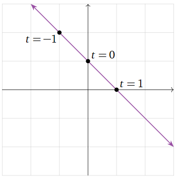
Figure 1.1.14
Now consider the system of two linear equations
{x+y+z=1x−z=0.
of Example 1.1.11. These collectively form the implicit equations for a line in R3. (At least two equations are needed to define a line in space.) This line also has a parametric form with one parameter t:
(x,y,z)=(t,1−2t,t).
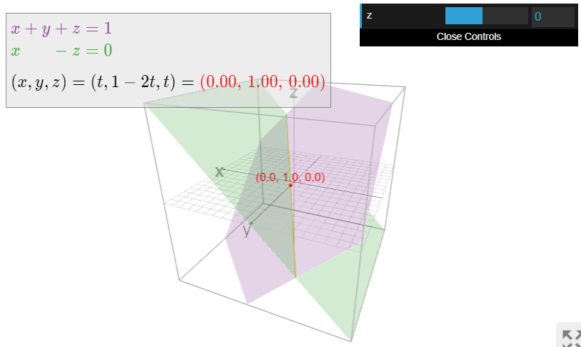
Note that in each case, the parameter t allows us to use R to label the points on the line. However, neither line is the same as the number line R: indeed, every point on the first line has two coordinates, like the point (0,1), and every point on the second line has three coordinates, like (0,1,0).
Consider the linear equation x+y+z=1 of Example 1.1.9. This is an implicit equation of a plane in space. This plane has an equation in parametric form: we can write every point on the plane as
(x,y,z)=(1−t−w,t,w)for anyt,w∈R.
In this case, we need two parameters t and w to describe all points on the plane.
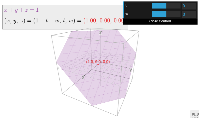
Note that the parameters t,w allow us to use R2 to label the points on the plane. However, this plane is not the same as the plane R2: indeed, every point on this plane has three coordinates, like the point (0,0,1).
When there is a unique solution, as in Example 1.1.10, it is not necessary to use parameters to describe the solution set.


